Introduction
rsgrad is an open-source command-line tool to help VASP players play better with VASP.
rsgrad is written proudly in pure Rust.
Now rsgrad provides several features:
- Track the relaxation and MD (molecular dynamics) progress;
- Calculate and visualize the DOS (density of states) and pDOS (projected DOS);
- Plot and visualize the band structure and fat band structure;
- Save the frames with given MD or relaxation trajectory;
- Calculate charge density difference;
- Analyze the vibration eigen values and eigen vectors;
- Plot the wave function at given bands in real-space;
- Plot the wave function at given bands in real-space then integrate it over specified plane;
- Plot and visualize the work function;
- Split POSCAR;
Convert between fractional coordinates and Cartesian coordinates;
Format POSCAR; - Generate POTCAR according to POSCAR;
- Calculate Transition Dipole Moment from WAVECAR;
- Calculate band gap and print locations of CBM and VBM.
- Convert one quantity to other units that representing same energy.
- Calculate the model non-adiabatic coupling for NAMD-LMI (a subset of Hefei-NAMD)
Wish you have a good time with rsgrad ^_^
Installation
There are two ways to install rsgrad, downloading the pre-built binaries and building from scratch.
Download the Binary from GitHub Release
We provide the pre-built binaries at GitHub Release.
There are four platforms we support with pre-built binaries
-
rsgrad-<VERSION>-linux-x86_64-musl.tar.gz: Statically linked binary. Can run on almost all Linux distros. However, themusl libcmay have performance issues in some scenes likewave1d,wav3detc. -
rsgrad-<VERSION>-linux-x86_64.tar.gz: Dynamically linked againstglibcand other fundamental system libraries.
For the binaries with 0.3.6_ci-test or upper version, they can run on most Linux distros (e.g. CentOS 7, Ubuntu 18.04).
If it still complains with message like/lib64/libc.so.6: version 'GLIBC_2.18' not found, just switch to-muslbinary or build from scratch. -
rsgrad-<VERSION>-macos-x86_64.tar.gz: Binary for macOS (Intel).rsgradis developed on macOS 13, which means you are don't need to worry about the availability if you are using macOS. -
rsgrad-<VERSION>-macos-aarch64.tar.gz: Binary for macOS (Apple Silicon). -
rsgrad-<VERSION>-windows-x86_64.zip: Binary for Windows system. We have no plan to support 32-bit systems.
Download the corresponding binary and put it in $PATH (or %PATH% on Windows), and have fun!
Build from Scratch
The build requires Internet accessibility.
-
If you haven't installed Rust toolchain, run
curl --proto '=https' --tlsv1.2 -sSf https://sh.rustup.rs | shand follow the instructions to configure it. When you finished the toolchain installation, you should be able to runcargoin command-line. Detailed instructions can be found here. -
If you have installed Rust toolchain already, just run
cargo install --git https://github.com/Ionizing/rsgrad. Several minutes later, thersgradshould be installed to~/.cargo/bin, no need to modify the$PATH(or%PATH%on Windows).
Relaxation
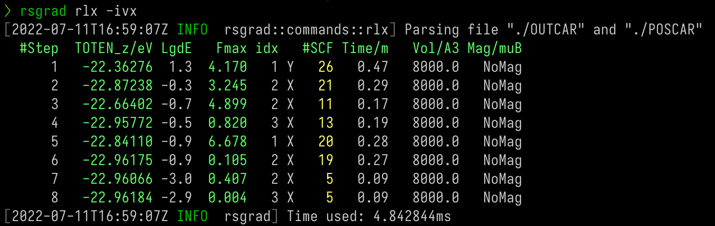
To track the relaxation or MD process, use rsgrad rlx. This command is useful if you want to know the progress
of geometry optimization (aka relaxation) or molecular dynamics.
This commands extract the following tags from OUTCAR:
- TOTEN
- TOTEN without entropy
- TOTEN difference between two ionic steps
- Maximum of atom forces (The negative EDIFFG is the threshold of this tag)
- The index of the atom with the maximum of force
- Number of SCF steps of each ionic step
- Time usage of each ionic step
- Volume of the cell
- Total magnetic moment
Help Message
$ rsgrad rlx -h
rsgrad-rlx
Tracking relaxation or MD progress

USAGE:
    rsgrad rlx [OPTIONS] [OUTCAR]

ARGS:
    <OUTCAR>    Specify the input OUTCAR file [default: ./OUTCAR]

OPTIONS:
    -a, --favg               Prints averaged total force in eV/A
    -e, --toten              Prints TOTEN in eV
    -h, --help               Print help information
    -i, --fmidx              Prints the index of ion with maximum total force load. Starts from 1
        --no-fmax            Don't print maximum total force in A^3
        --no-lgde            Don't print Log10(delta(TOTEN without entropy))
        --no-magmom          Don't print total magnetic moment in muB
        --no-nscf            Don't print number of SCF iteration for each ionic step
        --no-time            Don't print time elapsed for each ionic step in minutes
        --no-totenz          Don't print TOTEN without entropy in eV
    -p, --poscar <POSCAR>    Specify the input POSCAR file [default: ./POSCAR]
    -v, --volume             Prints lattice volume in A^3
    -x, --fmaxis             Prints the axis where the strongest total force component lies on.
                             [XYZ]
Example
Density of States
The rsgrad dos command calculates the Density of States (DOS) of current system.
rsgrad DOES NOT read the DOSCAR, but calculates the DOS from PROCAR instead by
$$ D(E) = \frac{1}{V} \sum_{i=1}^{N} \delta(E-E(\mathbf{k}_i)) $$
Because rsgrad uses arbitrary unit, the factor \(\frac{1}{V}\) is omitted. The \(\delta(x)\)
is replaced by Gaussian function or Lorentzian function:
$$ g(x) = \frac{1}{\sigma\sqrt{2\pi}} \exp \left( -\frac{1}{2} \frac{(x-\mu)^2}{\sigma^2} \right) \\ l(x) = \frac{1}{\pi} \frac{\sigma}{(x-\mu)^2 + \sigma^2} $$
where \(\mu\) is \(E(\mathbf{k}_i)\) and \(\sigma\) is sigma of configuration in the implementation.
This method makes it easier to calculate projected DOS with projection of specific atoms, angular moments and k-points.
However, this method sometimes differs from DOSCAR with ISMEAR = -5. For detailed explaination, see the
document here.
The OUTCAR is also needed to get the Fermi level.
Help Message
$ rsgrad dos -h
rsgrad-dos
Calculate density of states from PROCAR and OUTCAR

USAGE:
    rsgrad dos [OPTIONS]

OPTIONS:
    -c, --config <CONFIG>       Projected DOS configuration file path
        --gen-template          Generate projected DOS configuration template
    -h, --help                  Print help information
        --htmlout <HTMLOUT>     Save the projected DOS plot as HTML. Then you can view it in the
                                browser [default: dos.html]
        --outcar <OUTCAR>       OUTCAR path [default: ./OUTCAR]
        --procar <PROCAR>       PROCAR path [default: ./PROCAR]
        --show                  Open the browser and show the plot immediately
        --show-brief            Print brief info of PROCAR, this may be helpful when you write the
                                configuration
        --to-inline-html        Render the plot and print the rendered code to stdout
        --txtout <TXTOUT>       Save the raw data of projected DOS. Then you can replot it with more
                                advanced tools [default: dos_raw.txt]
        --xlim <XLIM> <XLIM>    Set the x-range of the plot [default: -1 6]
Configuration Template
The configuration template can be generated by running rsgrad dos --gen-template. The following configuration
is written to pband.toml by default:
# rsgrad DOS configuration in toml format.
# multiple tokens inside string are seperated by whitespace
method      = "Gaussian"        # smearing method
sigma       = 0.05              # smearing width, (eV)
procar      = "PROCAR"          # PROCAR path
outcar      = "OUTCAR"          # OUTCAR path
txtout      = "dos_raw.txt"     # save the raw data as "dos_raw.txt"
htmlout     = "dos.html"        # save the pdos plot as "dos.html"
totdos      = true              # plot the total dos
fill        = true              # fill the plot to x axis or not
xlim        = [-1, 6]           # x-range of plot

[pdos.plot1]                  # One label produces one plot, the labels CANNOT be repetitive.
                              # This label is 'plot1', to add more pdos, write '[pdos.plot2]' and so on.
kpoints = "1 3..7 -1"         # selects 1 3 4 5 6 7 and the last kpoint for pdos plot.
atoms   = "1 3..7 -1"         # selects 1 3 4 5 6 7 and the last atoms' projection for pdos plot.
orbits  = "s px dxy"          # selects the s px and dx orbits' projection for pdos plot.
factor  = 1.01                # the factor multiplied to this pdos

[pdos.plot2]                  # One label produces one plot, the labels CANNOT be repetitive.
                              # This label is 'plot2', to add more pdos, write '[pdos.plot2]' and so on.
kpoints = "1 3..7 -1"         # selects 1 3 4 5 6 7 and the last kpoint for pdos plot.
atoms   = "1 3..7 -1"         # selects 1 3 4 5 6 7 and the last atoms' projection for pdos plot.
orbits  = "s px dxy"          # selects the s px and dx orbits' projection for pdos plot.
factor  = 1.01                # the factor multiplied to this pdos

# The fields can be left blank, if you want select all the components for some fields,
# just comment them. You can comment fields with '#'
Example (without configuration file)
This command can calculate total DOS only. To calculate projected DOS, use configuration instead (see next section).
$ rsgrad dos
[2022-07-14T18:42:55Z INFO  rsgrad::commands::dos] Parsing PROCAR file "./PROCAR"
[2022-07-14T18:42:55Z INFO  rsgrad::commands::dos] Parsing OUTCAR file "./OUTCAR" for Fermi level
[2022-07-14T18:42:55Z INFO  rsgrad::commands::dos] Found Fermi level = -1.9018, eigenvalues will be shifted.
[2022-07-14T18:42:55Z INFO  rsgrad::commands::dos] Plotting Total DOS ...
[2022-07-14T18:42:55Z INFO  rsgrad::commands::dos] Total DOS plot time usage: 29.055µs
[2022-07-14T18:42:55Z INFO  rsgrad::commands::dos] Writing DOS plot to "dos.html"
[2022-07-14T18:42:55Z INFO  rsgrad::commands::dos] Writing raw DOS data to "dos_raw.txt"
[2022-07-14T18:42:55Z INFO  rsgrad] Time used: 124.426652ms
The output html should be like something in the following
Example (with configuration file)
To plot multiple PDOS, using configuration file is suggested.
With the configuration (pdos.toml) in the following
method      = "Gaussian"
sigma       = 0.05
procar      = "PROCAR"
outcar      = "OUTCAR"
txtout      = "dos_raw.txt"
htmlout     = "dos.html"
totdos      = true
fill        = true
xlim        = [-1, 6]

[pdos.Benzene]
atoms   = "37..48"

[pdos.AgSurf]
atoms   = "3 6 10 14 21 23 25 33 36"
then rsgrad dos -c pdos.toml
$ rsgrad dos -c pdos.toml
[2022-07-14T18:43:34Z INFO  rsgrad::commands::dos] Reading PDOS configuration from Some("pdos.toml")
[2022-07-14T18:43:34Z INFO  rsgrad::commands::dos] Parsing PROCAR file "PROCAR"
[2022-07-14T18:43:34Z INFO  rsgrad::commands::dos] Parsing OUTCAR file "OUTCAR" for Fermi level
[2022-07-14T18:43:34Z INFO  rsgrad::commands::dos] Found Fermi level = -1.9018, eigenvalues will be shifted.
[2022-07-14T18:43:34Z INFO  rsgrad::commands::dos] Plotting Total DOS ...
[2022-07-14T18:43:34Z INFO  rsgrad::commands::dos] Total DOS plot time usage: 42.878µs
[2022-07-14T18:43:34Z INFO  rsgrad::commands::dos] Plotting PDOS ...
[2022-07-14T18:43:34Z INFO  rsgrad::commands::dos] PDOS plot time usage: 6.223076ms
[2022-07-14T18:43:34Z INFO  rsgrad::commands::dos] Writing DOS plot to "dos.html"
[2022-07-14T18:43:34Z INFO  rsgrad::commands::dos] Writing raw DOS data to "dos_raw.txt"
[2022-07-14T18:43:34Z INFO  rsgrad] Time used: 61.982958ms
you will get something in the following
Usage of txtout
rsgrad can write the raw data of plot by setting txtout (dos_raw.txt by default). The organization of it
shows the energy, total DOS and projected dos respectively:
# E-Ef TotDOS Benzene AgSurf
...
        -7.921938         0.002969         0.002158         0.000004
        -7.899296         0.016032         0.011655         0.000019
        -7.876654         0.070713         0.051408         0.000085
        -7.854012         0.254749         0.185212         0.000307
        -7.831371         0.749573         0.544998         0.000910
        -7.808729         1.801235         1.309709         0.002202
        -7.786087         3.534640         2.570233         0.004349
        -7.763446         5.663677         4.118580         0.007011
        -7.740804         7.409459         5.388357         0.009226
        -7.718162         7.913407         5.755104         0.009908
        -7.695520         6.898991         5.017578         0.008683
        -7.672879         4.909619         3.570876         0.006208
        -7.650237         2.854880         2.076535         0.003622
        -7.627595         1.373037         0.998928         0.001724
        -7.604953         0.617183         0.449840         0.000672
        -7.582312         0.494734         0.362904         0.000231
        -7.559670         0.977346         0.718873         0.000173
        -7.537028         2.169137         1.593003         0.000599
        -7.514387         4.077126         2.981347         0.002383
        -7.491745         6.295459         4.560748         0.007858
        -7.469103         8.005154         5.685401         0.021128
...
The first line shows the labels of each series and have a hastag # in the beginning in order to let numpy.loadtxt
can read it directly.
Then you can throw it into other plotters like Excel, Matplotlib, OriginPro GnuPlot etc. and do whatever fancy things you prefer.
Band Structure
rsgrad band can plot the band structure from PROCAR and OUTCAR.
Help Message
$ rsgrad band -h
rsgrad-band
Plot bandstructure and projected bandstructure

USAGE:
    rsgrad band [OPTIONS]

OPTIONS:
    -c, --config <CONFIG>
            Band structure plot configuration file path

        --colormap <COLORMAP>
            [default: jet]

        --efermi <EFERMI>
            Set the E-fermi given from SCF's OUTCAR and it will be the reference energy level

        --gen-template
            Generate band structure plot configuration template

    -h, --help
            Print help information

        --htmlout <HTMLOUT>
            Save the band structure plot as HTML [default: band.html]

    -k, --kpoint-labels <KPOINT_LABELS>
            Symbols for high symmetry points on the kpoint path

        --ncl-spinor <NCL_SPINOR>
            [possible values: X, Y, Z]

        --outcar <OUTCAR>
            OUTCAR path [default: ./OUTCAR]

        --procar <PROCAR>
            PROCAR path [default: ./PROCAR]

        --show
            Open the browser and show the plot immediately

        --to-inline-html
            Render the plot and print the rendered code to stdout

        --txtout-prefix <TXTOUT_PREFIX>
            Save the raw data of band structure [default: band_raw]

        --ylim <YLIM> <YLIM>
            Set the y-range of the plot [default: "-1 6"]
Configuration Template
# rsgrad Band plot configuration in toml format.
# multiple tokens inside string are seperated by whitespace, if you

# kpoint-labels   = ["G", "K", "M", "G"]   # should be consistant with the boundaries in KPOINTS
procar          = "PROCAR"
outcar          = "OUTCAR"
txtout-prefix   = "band_raw"
htmlout         = "band.html"
# segment-ranges  = [[1, 40], [41, 80], [81, 120]]  # if commented, rsgrad will find the boundaries by judging if k[i] == k[i+1]
# ncl-spinor      = "Z"     # for vasp_ncl calculation
# colormap        = "jet"     # the colormap specified to plot ncl-band
# efermi          = 0.0       # if commented, rsgrad will read the efermi from OUTCAR, but if may be slightly different from scf's
# ylim            = [-1, 6]

# [pband.plot1]
# spins   = "up down"     # "u d" are also ok, for ncl system, "tot x y z" are available
# atoms   = "1 3..7 -1"   # which atoms to project on, if commented, all atoms are selected
# orbits  = "s px dxy"    # which orbits to project on, if commented, all orbits are selected
# color   = "red"         # the color of marker
Example (without configuration file)
Simply run rsgrad band can plot the band structure.
$ rsgrad band
[2022-07-14T18:40:18Z INFO  rsgrad::commands::band] Reading fermi level and lattice data from "./OUTCAR"
[2022-07-14T18:40:18Z INFO  rsgrad::commands::band] Reading band data from "./PROCAR"
[2022-07-14T18:40:18Z INFO  rsgrad::commands::band] Found Fermi level: 12.7626, shifting eigenvalues ...
[2022-07-14T18:40:18Z WARN  rsgrad::commands::band] No k-point labels found, use empty labels instead
[2022-07-14T18:40:18Z INFO  rsgrad::commands::band] Plotting raw bands ...
[2022-07-14T18:40:18Z INFO  rsgrad::commands::band] Writing Bandstructure to "band.html"
[2022-07-14T18:40:18Z INFO  rsgrad::commands::band] Writing raw band data to "band_raw.txt"
[2022-07-14T18:40:18Z INFO  rsgrad] Time used: 79.644034ms
There may be a warning reminds you provide the labels of each high-symmetry point.
rsgrad identifies high-symmetry points by calculate the difference of consecutive k-points.
If the difference equals zero, these two points are labelled as one high-symmetry point.
For example:
...
k-point    38 :       0.0000    0.0256    0.0000
k-point    39 :       0.0000    0.0128    0.0000
k-point    40 :       0.0000    0.0000    0.0000
k-point    41 :       0.0000    0.0000    0.0000
k-point    42 :      -0.0085    0.0171    0.0000
k-point    43 :      -0.0171    0.0342    0.0000
...
k-point 40 and k-point 41 are same, thus be identified as one high-symmetry point. Each of the high-symmetry
points need a label. You may either left the --kpoint-labels empty or provide the correct labels seperated
by white spaces. Sometimes it may produce wrong band structure due to the special k-point path like
kpoints for bandstructure L-G-X-U K-G
 10
line
reciprocal
  0.50000  0.50000  0.50000    1
  0.00000  0.00000  0.00000    1

  0.00000  0.00000  0.00000    1
  0.00000  0.50000  0.50000    1

  0.00000  0.50000  0.50000    1
  0.25000  0.62500  0.62500    1

  0.37500  0.7500   0.37500    1
  0.00000  0.00000  0.00000    1
The end of third segment (0.25000, 0.62500, 0.62500) and the beginning of fourth segment (0.37500, 0.7500, 0.37500) are not consistent, which produces wrong k-path, leading to wrong band structure:
To solve this issue, you need to try the configuration file.
Example (with configuration file)
With the configuration in the following
kpoint-labels   = ["L", "Γ", "X", "U|K", "Γ"]
procar          = "PROCAR"
outcar          = "OUTCAR"
txtout-prefix   = "pband_raw"
htmlout         = "pband.html"
segment-ranges  = [[1, 10], [11, 20], [21, 30], [31, 40]]

[pband.Si-p-orbit]
orbits  = "px py pz"
color   = "red"
factor  = 2.0
and run rsgrad -c pband.toml
$ rsgrad band -c pband.toml
[2022-07-14T18:41:02Z INFO  rsgrad::commands::band] Reading porjected band configuration fomr Some("pband.toml")
[2022-07-14T18:41:02Z INFO  rsgrad::commands::band] Reading fermi level and lattice data from "OUTCAR"
[2022-07-14T18:41:02Z INFO  rsgrad::commands::band] Reading band data from "PROCAR"
[2022-07-14T18:41:02Z INFO  rsgrad::commands::band] Found Fermi level: 12.7626, shifting eigenvalues ...
[2022-07-14T18:41:02Z INFO  rsgrad::commands::band] Plotting raw bands ...
[2022-07-14T18:41:02Z INFO  rsgrad::commands::band] Plotting projected bands ...
[2022-07-14T18:41:02Z INFO  rsgrad::commands::band] Writting projected band Si-p-orbit to "pband_raw_Si-p-orbit.txt" ...
[2022-07-14T18:41:02Z INFO  rsgrad::commands::band] Projected band plot time usage: 1.220401ms
[2022-07-14T18:41:02Z INFO  rsgrad::commands::band] Writing Bandstructure to "band.html"
[2022-07-14T18:41:02Z INFO  rsgrad::commands::band] Writing raw band data to "pband_raw.txt"
[2022-07-14T18:41:02Z INFO  rsgrad] Time used: 77.804627ms
then it produces
Example (for non-collinear system)
For the results produced by vasp_ncl, rsgrad supports plotting the \(z\) (\(x\) and \(y\) are also OK) projection to
analyze the spin angular moments.
kpoint-labels   = ["M", "Γ", "K", "M"]
procar          = "PROCAR"
outcar          = "OUTCAR"
txtout-prefix   = "band_ncl_raw"
htmlout         = "band_ncl.html"
segment-ranges  = [[81, 120], [1, 40], [41, 80]]
ncl-spinor      = "Z"
colormap        = "jet"
then it produces
Trajectory
rsgrad reads OUTCAR then provide some operations in the following.
- Save selected steps as XDATCAR.
- Save selected steps as POSCAR files.
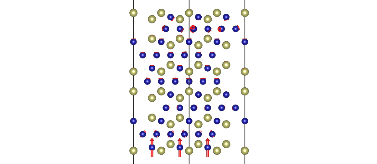
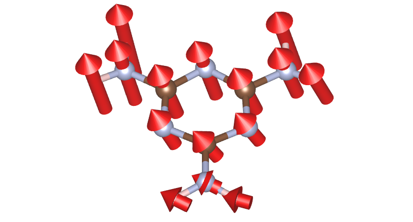
- Save selected steps as XSF files. With XSF, VESTA can show the force vectors on every atom.
Help Message
$ rsgrad traj --help
rsgrad-traj
Operations about relaxation/MD trajectory.

POSCAR is needed if you want to preserve the constraints when saving frames to POSCAR.

USAGE:
    rsgrad traj [OPTIONS] [--] [OUTCAR]

ARGS:
    <OUTCAR>
            Specify the input OUTCAR file

            [default: ./OUTCAR]

OPTIONS:
        --cartesian
            Save to POSCAR in cartesian coordinates, the coordinates written is direct/fractional by
            default

    -d, --save-as-xdatcar
            Save whole trajectory in XDATCAR format

    -h, --help
            Print help information

    -i, --select-indices <SELECT_INDICES>...
            Selects the indices to operate.

            Step indices start from '1', if '0' is given, all the structures will be selected. Step
            indices can be negative, where negative index means counting reversely. E.g.
            "-i -2 -1 1 2 3" means selecting the last two and first three steps.

        --no-add-symbol-tags
            Don't add chemical symbol to each line of coordinates

        --no-preserve-constraints
            Don't preverse constraints when saving trajectory to POSCAR

    -p, --poscar <POSCAR>
            Specify the input POSCAR file

            [default: ./POSCAR]

    -s, --save-as-poscar
            Save selected steps as POSCARs

        --save-in <SAVE_IN>
            Define where the files would be saved

            [default: .]

    -x, --save-as-xsfs
            Saves each selected modes to XSF file, this file includes each atom's force information
Examples
- Take the last step and save as XSF file
rsgrad traj -i -1 -x
$ rsgrad traj -i -1 -x
[2022-07-14T18:37:35Z INFO  rsgrad::commands::traj] Parsing file "./OUTCAR" and "./POSCAR"
[2022-07-14T18:37:35Z INFO  rsgrad::vasp_parsers::outcar] Saving ionic step to "./step_0003.xsf" ...
[2022-07-14T18:37:35Z INFO  rsgrad] Time used: 11.223561ms
- Take the first step and save as POSCAR file
rsgrad traj -i 1 -s
$ rsgrad traj -i 1 -s
[2022-07-14T18:38:51Z INFO  rsgrad::commands::traj] Parsing file "./OUTCAR" and "./POSCAR"
[2022-07-14T18:38:51Z INFO  rsgrad::vasp_parsers::outcar] Saving trajectory step #    1 to "./POSCAR_00001.vasp" ...
[2022-07-14T18:38:51Z INFO  rsgrad] Time used: 8.64197ms
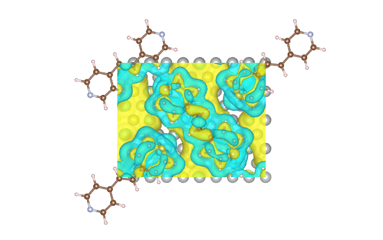
Charge Density Difference
rsgrad chgdiff can calculate the charge density difference from CHGCAR files:
$$ \Delta \rho = \rho_{A+B} - (\rho_A + \rho_B) $$
Where \(\rho_{A+B}\), \(\rho_A\) and \(\rho_B\) are the charge densities of total structure, A structure and B structure, respectively.
You may also need rsgrad poscar --split ... to generate
the structure of A and B from A+B.
Help message
$ rsgrad chgdiff --help
rsgrad-chgdiff
Calculate charge density difference.

The operation is performed by `chgdiff = chgcar_ab - (chgcar_a + chgcar_b)`.

USAGE:
    rsgrad chgdiff [OPTIONS] <CHGCAR_AB> <CHGCAR_A> <CHGCAR_B>

ARGS:
    <CHGCAR_AB>
            The CHGCAR of A+B system

    <CHGCAR_A>
            The CHGCAR of A system

    <CHGCAR_B>
            The CHGCAR of B system

OPTIONS:
    -h, --help
            Print help information

    -o, --output <OUTPUT>
            The output charge density difference file path

            [default: CHGDIFF.vasp]
Example
You need to calculate the electronic structure of the three structures (A+B, A and B) first,
then rsgrad chgdiff CHGCAR_A+B CHGCAR_A CHGCAR_B like
$ rsgrad chgdiff ../scf/CHGCAR Ag/CHGCAR noAg/CHGCAR
[2022-07-14T18:34:59Z INFO  rsgrad::commands::chgdiff] Reading charge density from "Ag/CHGCAR"
[2022-07-14T18:34:59Z INFO  rsgrad::commands::chgdiff] Reading charge density from "noAg/CHGCAR"
[2022-07-14T18:34:59Z INFO  rsgrad::commands::chgdiff] Reading charge density from "../scf/CHGCAR"
[2022-07-14T18:35:06Z INFO  rsgrad::commands::chgdiff] Calculating charge density difference by `CHGDIFF = "../scf/CHGCAR" - ("Ag/CHGCAR" + "noAg/CHGCAR")`
[2022-07-14T18:35:06Z INFO  rsgrad::commands::chgdiff] Writing charge difference to "CHGDIFF.vasp"
[2022-07-14T18:35:10Z INFO  rsgrad] Time used: 11.189259653s
finally use VESTA to visualize the data
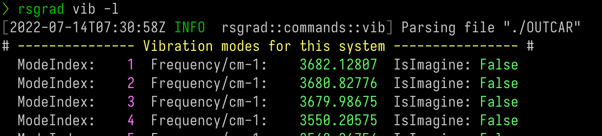
Vibration
For systems enabled vibration calculation (phonon at Γ point only), rsgrad vib can
- Print the phonon eigenvalues;
- Save the phonon eigenvectors;
- Modulate the ground-state according to specified modes.
Help Message
$ rsgrad vib --help
rsgrad-vib
Tracking vibration information.

For systems enabled vibration mode calculation, this command can extract phonon eigenvalues and
phonon eigenvectors at Gamma point.

USAGE:
    rsgrad vib [OPTIONS] [--] [OUTCAR]

ARGS:
    <OUTCAR>
            Specify the input OUTCAR file

            [default: ./OUTCAR]

OPTIONS:
    -a, --amplitude <AMPLITUDE>
            Modulation amplitude coefficient, to avoid precision issue, abs(amplitude) >= 0.01
            should be satisfied

            [default: 0.1]

    -c, --cartesian
            Catesian coordinate is used when writting POSCAR. Fractional coordinate is used by
            default

    -h, --help
            Print help information

    -i, --select-indices <SELECT_INDICES>...
            Selects the mode indices to operate.

            Step indices start from '1', if '0' is given, all the structures will be selected. Step
            indices can be negative, where negative index means counting reversely. E.g. "-i -2 -1 1
            2 3" means selecting the last two and first three steps.

    -l, --list
            Shows vibration modes in brief

    -m, --modulate
            Modulate the ground-state POSCAR with respect to a certern vibration frequencies

    -p, --poscar <POSCAR>
            Specify the input POSCAR file, the consntraints info is needed

            [default: ./POSCAR]

        --save-in <SAVE_IN>
            Define where the files would be saved

            [default: .]

    -x, --save-as-xsfs
            Saves each selected modes to XSF file
Example
-
Print the phonon eigenvalues;
-
Save the phonon eigenvectors;
$ rsgrad vib -i {1..3} {-3..-1} -x
[2022-07-14T18:32:49Z INFO  rsgrad::commands::vib] Parsing file "./OUTCAR"
[2022-07-14T18:32:49Z INFO  rsgrad::vasp_parsers::outcar] Saving mode #   1 as "./mode_0001_3682.13cm-1.xsf" ...
[2022-07-14T18:32:49Z INFO  rsgrad::vasp_parsers::outcar] Saving mode #   3 as "./mode_0003_3679.99cm-1.xsf" ...
[2022-07-14T18:32:49Z INFO  rsgrad::vasp_parsers::outcar] Saving mode #  44 as "./mode_0044_0010.79cm-1_imag.xsf" ...
[2022-07-14T18:32:49Z INFO  rsgrad::vasp_parsers::outcar] Saving mode #  43 as "./mode_0043_0007.12cm-1_imag.xsf" ...
[2022-07-14T18:32:49Z INFO  rsgrad::vasp_parsers::outcar] Saving mode #   2 as "./mode_0002_3680.83cm-1.xsf" ...
[2022-07-14T18:32:49Z INFO  rsgrad::vasp_parsers::outcar] Saving mode #  45 as "./mode_0045_0047.20cm-1_imag.xsf" ...
[2022-07-14T18:32:49Z INFO  rsgrad] Time used: 109.566967ms
- Modulate the ground-state according to specified modes.
$ rsgrad vib -i {-3..-1} --modulate --amplitude 0.1
[2022-07-14T18:31:41Z INFO  rsgrad::commands::vib] Parsing file "./OUTCAR"
[2022-07-14T18:31:41Z INFO  rsgrad::vasp_parsers::outcar] Saving modulated POSCAR of mode #  43 with amplitude coeff 0.100 as "./mode_0043_0007.12cm-1_0.100_imag.vasp" ...
[2022-07-14T18:31:41Z INFO  rsgrad::vasp_parsers::outcar] Saving modulated POSCAR of mode #  44 with amplitude coeff 0.100 as "./mode_0044_0010.79cm-1_0.100_imag.vasp" ...
[2022-07-14T18:31:41Z INFO  rsgrad::vasp_parsers::outcar] Saving modulated POSCAR of mode #  45 with amplitude coeff 0.100 as "./mode_0045_0047.20cm-1_0.100_imag.vasp" ...
[2022-07-14T18:31:41Z INFO  rsgrad] Time used: 202.629805ms
Wavefunction 3D
Main functions of rsgrad wav3d
- List the brief information of WAVECAR;
- Save the selected pseudo-wavefunction to .vasp file;
- Reconstruct and save the all-electron wavefunction with
--ae.
Help Message
$ rsgrad wav3d --help
Plot wavefunction in realspace, and save it as '.vasp' file

Usage: rsgrad wav3d [OPTIONS]

Options:
  -w, --wavecar <WAVECAR>
          WAVECAR file name

          [default: ./WAVECAR]

  -p, --poscar <POSCAR>
          POSCAR filename, POSCAR is needed to get the real-space wavefunction

          [default: ./POSCAR]

      --potcar <POTCAR>
          POTCAR filename, required when reconstructing all-electron wavefunctions

          [default: ./POTCAR]

  -s, --ispins [<ISPINS>...]
          Select spin index, starting from 1

          [default: 1]

  -k, --ikpoints [<IKPOINTS>...]
          Select kpoint index, starting from 1.

          You can input ranges directly: `-k 1..4 5..10`

          [default: 1]

  -b, --ibands [<IBANDS>...]
          Select band index, starting from 1.

          You can input ranges directly: `-b 1..4 5..10`

  -l, --list
          List the brief info of current WAVECAR

  -d, --detail
          Show the eigen values and band occupations of current WAVECAR.

          This flag should be used with `--list`

      --gamma-half <GAMMA_HALF>
          Gamma Half direction of WAVECAR. You need to set this to 'x' or 'z' when processing WAVECAR produced by `vasp_gam`

          [possible values: x, z]

      --ae
          Reconstruct the all-electron wavefunction instead of using the pseudo-wavefunction

      --aecut <AECUT>
          AE energy cutoff in eV. Negative values mean |aecut| * pscut

          [default: -2]

      --ngrid <NGRID> <NGRID> <NGRID>
          Grid size for realspace wavefunction, 3 numbers are required, i.e. NGXF NGYF and NGZF.

          If this argument is left empty, NG_F will be set as NG_F=2*NG_.

          Be aware that NG_F must be greater than or at least equal to corresponding NG_.

  -o, --output-parts [<OUTPUT_PARTS>...]
          Specify output part of the wavefunction.

          Detailed message:
           - normsquared/ns: Perform `ρ(r) = |ѱ(r)|^2` action to get the spatial distribution of selected band.
           - real/re: Real part of the wavefunction, suffix '_re.vasp' is added to the output filename.
           - imag/im: Imaginary part of the wavefunction, suffix '_im.vasp' is added to the output filename.
           - reim: Output both real part and imaginary parts of the wavefunction.
           - uns/dns: Perform `ρ(r) = |ѱ(r)|^2` for spinor up/down only. **Note: this option works for `ncl` WAVECAR only.**

          [possible values: normsquared, ns, uns, dns, real, re, imag, im, reim]

      --prefix <PREFIX>
          Prefix of output filename

          [default: wav]

  -e, --show-eigs-suffix
          Add eigen value suffix to the filename

      --sum-chgs
          Perform sum-up of the charge densities for selected bands.

          With this flag open, only `normsquared` or `ns` or `uns` or `dns` are allowed for the `-o`/`--output-parts` option.
           IMPORTANT NOTES:
           - The prefix for output filename `sum-prefix` is also required and has no default prefix.
           - The individual charge densities will not be saved to corresponding '.vasp' files if this flag is on.

      --sum-prefix <SUM_PREFIX>
          Specify the output file for the summed charge densities.

          This argument is required if `sum_chgs` is on.

  -h, --help
          Print help (see a summary with '-h')
Example
- List the brief information of WAVECAR
$ rsgrad wav3d -l

[2022-07-14T09:19:51Z INFO  rsgrad::commands::wav3d] Reading WAVECAR: "./WAVECAR"
LENGTH     =             54145104
RECLEN     =              1388336
TYPE       =             Standard
NSPIN      =                    1
NKPTS      =                    1
NBANDS     =                   36
ENCUT      =              450.000
EFERMI     =               -5.368
VOLUME     =             8000.000
NGRID      = [  71,   71,   71]
NPLWS      = [173541]
ACELL      = [[  20.000,    0.000,    0.000], [   0.000,   20.000,    0.000], [   0.000,    0.000,   20.000]]
BCELL      = [[   0.050,    0.000,    0.000], [   0.000,    0.050,    0.000], [   0.000,    0.000,    0.050]]


[2022-07-14T09:19:51Z INFO  rsgrad] Time used: 160.337862ms
if you want the band eigen values information
$ rsgrad wav3d -ld

...
<BRIEF INFORMATION ABOUT WAVECAR>
...

ISPIN:  1  IKPOINT:    1  IBAND:     1 E-Efermi:    -19.991 Occupation: 1.000
ISPIN:  1  IKPOINT:    1  IBAND:     2 E-Efermi:    -18.141 Occupation: 1.000
ISPIN:  1  IKPOINT:    1  IBAND:     3 E-Efermi:    -18.141 Occupation: 1.000
ISPIN:  1  IKPOINT:    1  IBAND:     4 E-Efermi:    -16.418 Occupation: 1.000
ISPIN:  1  IKPOINT:    1  IBAND:     5 E-Efermi:    -15.534 Occupation: 1.000
ISPIN:  1  IKPOINT:    1  IBAND:     6 E-Efermi:    -15.532 Occupation: 1.000
ISPIN:  1  IKPOINT:    1  IBAND:     7 E-Efermi:    -10.662 Occupation: 1.000
ISPIN:  1  IKPOINT:    1  IBAND:     8 E-Efermi:    -10.661 Occupation: 1.000
...
- Save the selected wavefunction to .vasp file
$ rsgrad wav3d -b {10..20} -o ns -e

[2022-07-14T09:23:06Z INFO  rsgrad::commands::wav3d] Reading WAVECAR: "./WAVECAR"
[2022-07-14T09:23:06Z INFO  rsgrad::commands::wav3d] Reading POSCAR: "./POSCAR"
[2022-07-14T09:23:06Z INFO  rsgrad::commands::wav3d] Processing spin 1, k-point   1, band   10 ...
[2022-07-14T09:23:06Z INFO  rsgrad::commands::wav3d] Processing spin 1, k-point   1, band   13 ...
[2022-07-14T09:23:06Z INFO  rsgrad::commands::wav3d] Processing spin 1, k-point   1, band   11 ...
[2022-07-14T09:23:06Z INFO  rsgrad::commands::wav3d] Processing spin 1, k-point   1, band   14 ...
[2022-07-14T09:23:06Z INFO  rsgrad::commands::wav3d] Processing spin 1, k-point   1, band   12 ...
[2022-07-14T09:23:06Z INFO  rsgrad::commands::wav3d] Processing spin 1, k-point   1, band   15 ...
[2022-07-14T09:23:06Z INFO  rsgrad::commands::wav3d] Writing "wav_1-1-13_-5.740eV.vasp" ...
[2022-07-14T09:23:06Z INFO  rsgrad::commands::wav3d] Writing "wav_1-1-15_-5.601eV.vasp" ...
[2022-07-14T09:23:06Z INFO  rsgrad::commands::wav3d] Writing "wav_1-1-14_-5.728eV.vasp" ...
[2022-07-14T09:23:06Z INFO  rsgrad::commands::wav3d] Writing "wav_1-1-10_-8.376eV.vasp" ...
[2022-07-14T09:23:06Z INFO  rsgrad::commands::wav3d] Writing "wav_1-1-11_-7.385eV.vasp" ...
[2022-07-14T09:23:06Z INFO  rsgrad::commands::wav3d] Writing "wav_1-1-12_-7.380eV.vasp" ...
[2022-07-14T09:23:08Z INFO  rsgrad::commands::wav3d] Processing spin 1, k-point   1, band   18 ...
[2022-07-14T09:23:08Z INFO  rsgrad::commands::wav3d] Processing spin 1, k-point   1, band   19 ...
[2022-07-14T09:23:09Z INFO  rsgrad::commands::wav3d] Writing "wav_1-1-18_-3.514eV.vasp" ...
[2022-07-14T09:23:09Z INFO  rsgrad::commands::wav3d] Processing spin 1, k-point   1, band   16 ...
[2022-07-14T09:23:09Z INFO  rsgrad::commands::wav3d] Processing spin 1, k-point   1, band   20 ...
[2022-07-14T09:23:09Z INFO  rsgrad::commands::wav3d] Writing "wav_1-1-19_-3.265eV.vasp" ...
[2022-07-14T09:23:09Z INFO  rsgrad::commands::wav3d] Processing spin 1, k-point   1, band   17 ...
[2022-07-14T09:23:10Z INFO  rsgrad::commands::wav3d] Writing "wav_1-1-16_-5.477eV.vasp" ...
[2022-07-14T09:23:10Z INFO  rsgrad::commands::wav3d] Writing "wav_1-1-17_-3.546eV.vasp" ...
[2022-07-14T09:23:10Z INFO  rsgrad::commands::wav3d] Writing "wav_1-1-20_-0.701eV.vasp" ...
[2022-07-14T09:23:11Z INFO  rsgrad] Time used: 5.484733549s
Open the .vasp in VESTA
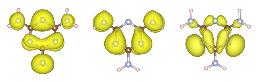
rsgrad wav3d supports extracting multiple bands at the same time, and the processes
executed in parallel, which can save a lot of time.
All-Electron Reconstruction
rsgrad aewfc has been merged into rsgrad wav3d.
Use --ae to reconstruct the all-electron wavefunction, and provide --potcar.
$ rsgrad wav3d --ae --potcar POTCAR -b 10 -o ns
If you also want the reconstructed real and imaginary parts, keep using -o re, -o im, or -o reim.
Current limitation: --ae is not available for non-collinear WAVECAR.
Wavefunction 1D
This command is similar to rsgrad wav3d. The only difference is that wav1d integrates
the wavefunction over specified plane, and produces the averaged one dimensional wavefunction.
It also supports all-electron reconstruction through --ae.
This command is useful when you are looking for image potential states.
Help Message
$ rsgrad wav1d --help
Plot wavefunction in realspace, then integrate over some plane, and save it as '.txt' file

Usage: rsgrad wav1d [OPTIONS]

Options:
  -w, --wavecar <WAVECAR>
          WAVECAR file name

          [default: ./WAVECAR]

  -s, --ispins [<ISPINS>...]
          Select spin index, starting from 1

          [default: 1]

  -k, --ikpoints [<IKPOINTS>...]
          Select kpoint index, starting from 1.

          You can input range directly: `-k 1..5 8..10`

          [default: 1]

  -b, --ibands [<IBANDS>...]
          Select band index, starting from 1.

          You can input range directly: `-b 5..10 14..19`

  -l, --list
          List the brief info of current WAVECAR

  -d, --detail
          Show the eigen values and band occupations of current WAVECAR.

          This flag should be used with `--list`

      --gamma-half <GAMMA_HALF>
          Gamma Half direction of WAVECAR. You need to set this to 'x' or 'z' when processing WAVECAR produced by `vasp_gam`

          [possible values: x, z]

      --poscar <POSCAR>
          POSCAR filename, required when reconstructing all-electron wavefunctions

          [default: ./POSCAR]

      --potcar <POTCAR>
          POTCAR filename, required when reconstructing all-electron wavefunctions

          [default: ./POTCAR]

      --ae
          Reconstruct the all-electron wavefunction density instead of using the pseudo-wavefunction

      --aecut <AECUT>
          AE energy cutoff in eV. Negative values mean |aecut| * pscut

          [default: -2]

      --txtout <TXTOUT>
          Specify the file name to be written with raw wav1d data

          [default: wav1d.txt]

      --htmlout <HTMLOUT>
          Specify the file name to be written with html wav1d data

          [default: wav1d.html]

      --axis <AXIS>
          Integration direction. e.g. if 'z' is provided, the XoY plane is integrated

          [default: z]
          [possible values: x, y, z]

      --to-inline-html
          Render the plot and print thw rendered code to stdout

      --show
          Open the browser and show the plot immediately

      --scale <SCALE>
          Scale the wavefunction

          [default: 10]

  -h, --help
          Print help (see more with '--help')
Example
The usage is similar to rsgrad wav3d, too.
$ rsgrad wav1d -b {20..27}
[2022-07-14T12:54:35Z INFO  rsgrad::commands::wav1d] Reading WAVECAR: "./WAVECAR"
[2022-07-14T12:54:36Z INFO  rsgrad::commands::wav1d] Processing spin 1, k-point   1, band   20 ...
[2022-07-14T12:54:36Z INFO  rsgrad::commands::wav1d] Processing spin 1, k-point   1, band   24 ...
[2022-07-14T12:54:36Z INFO  rsgrad::commands::wav1d] Processing spin 1, k-point   1, band   22 ...
[2022-07-14T12:54:36Z INFO  rsgrad::commands::wav1d] Processing spin 1, k-point   1, band   23 ...
[2022-07-14T12:54:36Z INFO  rsgrad::commands::wav1d] Processing spin 1, k-point   1, band   21 ...
[2022-07-14T12:54:36Z INFO  rsgrad::commands::wav1d] Processing spin 1, k-point   1, band   26 ...
[2022-07-14T12:54:36Z INFO  rsgrad::commands::wav1d] Processing spin 1, k-point   1, band   27 ...
[2022-07-14T12:54:36Z INFO  rsgrad::commands::wav1d] Processing spin 1, k-point   1, band   25 ...
[2022-07-14T12:54:36Z INFO  rsgrad::commands::wav1d] Writing to "wav1d.html"
[2022-07-14T12:54:36Z INFO  rsgrad::commands::wav1d] Writing to "wav1d.txt"
[2022-07-14T12:54:36Z INFO  rsgrad::commands::wav1d] Printing inline html to stdout ...
[2022-07-14T12:54:36Z INFO  rsgrad] Time used: 864.911523ms
Then produces
Note: The Fermi level is shiftted to 0.0 eV
All-Electron Reconstruction
rsgrad aewfc has been merged into rsgrad wav1d for 1D integrated output.
Use --ae --poscar POSCAR --potcar POTCAR to integrate the reconstructed all-electron density:
$ rsgrad wav1d --ae --poscar POSCAR --potcar POTCAR -b 20..27
Current limitation: --ae is not available for non-collinear WAVECAR.
Workfunction
rsgrad workfunc reads LOCPOT to calculate the work function. For further discussion about
work function, please read this blog.
Note: rsgrad workfunc does not show the vacuum level directly, hence you need to find it by
hovering on the step of the work function. Take the work function above as an example, the
vacuum level should be about 4.048eV around 40Å.
Help Message
$ rsgrad workfunc --help
rsgrad-workfunc
Calculate work-function from LOCPOT file, OUTCAR is also needed to get the Fermi level.

The work function is calculated by plannar integration of the data cube in LOCPOT. The selected axis
should be perpendicular to the other two axises.

USAGE:
    rsgrad workfunc [OPTIONS] [LOCPOT]

ARGS:
    <LOCPOT>
            LOCPOT file path. Turn on 'LVHAR' in INCAR to get the electro-static potential saved it

            [default: ./LOCPOT]

OPTIONS:
        --axis <AXIS>
            Integration direction. e.g. if 'z' is provided, the XoY plane is integrated

            [default: z]
            [possible values: X, Y, Z]

    -h, --help
            Print help information

    -o, --htmlout <HTMLOUT>
            Write the plot to html and view it in the web browser

            [default: ./workfunction.html]

        --outcar <OUTCAR>
            OUTCAR file path. This file is needed to get the E-fermi level and lattice properties

            [default: ./OUTCAR]

        --show
            Open default browser to see the plot immediately

        --to-inline-html
            Render the plot and print the rendered code to stdout

        --txtout <TXTOUT>
            Write the raw plot data as txt file in order to replot it with more advanced tools

            [default: locpot.txt]
Example
In general, you don't need t provide additional arguments.
$ rsgrad workfunc
[2022-07-14T14:41:38Z INFO  rsgrad::commands::workfunc] Reading "./OUTCAR"
[2022-07-14T14:41:38Z INFO  rsgrad::commands::workfunc] Reading electro-static potential data from "./LOCPOT"
[2022-07-14T14:41:39Z INFO  rsgrad::commands::workfunc] Writing raw plot data to "locpot.txt"
[2022-07-14T14:41:39Z INFO  rsgrad::commands::workfunc] Writing to "./workfunction.html"
[2022-07-14T14:41:39Z INFO  rsgrad] Time used: 1.352347116s
POSCAR
There are several operations that rsgrad pos can do
- Convert the fractional coordinates to Cartesian coordinates or convert reversely;
- Split the POSCAR and save the two parts;
This command is useful when you want to calculate charge density difference and adsorption energy. - Format the POSCAR and add element symbol tags to each atom.
Help Message
$ rsgrad pos --help
rsgrad-pos
Operation(s) about POSCAR, including split it into two POSCARs

USAGE:
    rsgrad pos [OPTIONS] [--] [POSCAR]

ARGS:
    <POSCAR>
            Specify the input POSCAR file

            [default: ./POSCAR]

OPTIONS:
    -a, --a-name <A_NAME>
            Splitted POSCAR path with selected atoms

            [default: POSCAR_A]

    -b, --b-name <B_NAME>
            Splitted POSCAR path with complement of `a_name`

            [default: POSCAR_B]

    -c, --cartesian
            Cartesian coordinates is used in writting POSCAR

        --convert
            Convert POSCAR to cartesian coordinates or fractional coordinates

        --converted <CONVERTED>
            The target path of converted POSCAR

            [default: POSCAR_new]

    -h, --help
            Print help information

    -i, --select-indices <SELECT_INDICES>...
            Selects the indices to operate.

            Step indices start from '1', if '0' is given, all the structures will be selected. Step
            indices can be negative, where negative index means counting reversely. E.g. "-i -2 -1 1
            2 3" means selecting the last two and the first three atom.

        --no-add-symbols-tags
            The symbols of each atom will not be written as comment in POSCAR

        --no-preserve-constraints
            Atom constraints will be dropped when writting POSCAR

    -s, --split
            Split POSCAR according to selected_indices
Examples
- Format the POSCAR to add element symbol tags
The original POSCAR of CO2:
 C  O
 1.0000000000000000
    20.0000000000000000    0.0000000000000000    0.0000000000000000
     0.0000000000000000   20.0000000000000000    0.0000000000000000
     0.0000000000000000    0.0000000000000000   20.0000000000000000
 C   O
   1   2
Direct
  0.5000000000000000  0.5000000000000000 -0.5000000000000000
  0.5754584707965210  0.4974961803083730  0.5000000000000000
  0.4249089651951450  0.5078477015701101  0.5000000000000000
Then run rsgrad pos POSCAR --convert
$ rsgrad pos POSCAR --convert
[2022-07-14T15:38:47Z INFO  rsgrad::commands::pos] Reading POSCAR file "POSCAR" ...
[2022-07-14T15:38:47Z INFO  rsgrad::commands::pos] Converting it to "POSCAR_new"
[2022-07-14T15:38:47Z INFO  rsgrad::commands::pos] Done
[2022-07-14T15:38:47Z INFO  rsgrad] Time used: 1.96796ms
The formatted file should be POSCAR_new
C  O
 1.0000000
      20.000000000       0.000000000       0.000000000
       0.000000000      20.000000000       0.000000000
       0.000000000       0.000000000      20.000000000
      C      O
      1      2
Direct
      0.5000000000      0.5000000000     -0.5000000000 !      C-001    1
      0.5754584708      0.4974961803      0.5000000000 !      O-001    2
      0.4249089652      0.5078477016      0.5000000000 !      O-002    3
- Convert POSCAR to Cartesian coordinates
Just run rsgrad pos POSCAR --convert --cartesian
$ rsgrad pos POSCAR --convert --cartesian
[2022-07-14T15:40:33Z INFO  rsgrad::commands::pos] Reading POSCAR file "POSCAR" ...
[2022-07-14T15:40:33Z INFO  rsgrad::commands::pos] Converting it to "POSCAR_new"
[2022-07-14T15:40:33Z INFO  rsgrad::commands::pos] Done
[2022-07-14T15:40:33Z INFO  rsgrad] Time used: 1.57861ms
The converted file POSCAR_new should be like
C  O
 1.0000000
      20.000000000       0.000000000       0.000000000
       0.000000000      20.000000000       0.000000000
       0.000000000       0.000000000      20.000000000
      C      O
      1      2
Cartesian
     10.0000000000     10.0000000000    -10.0000000000 !      C-001    1
     11.5091694159      9.9499236062     10.0000000000 !      O-001    2
      8.4981793039     10.1569540314     10.0000000000 !      O-002    3
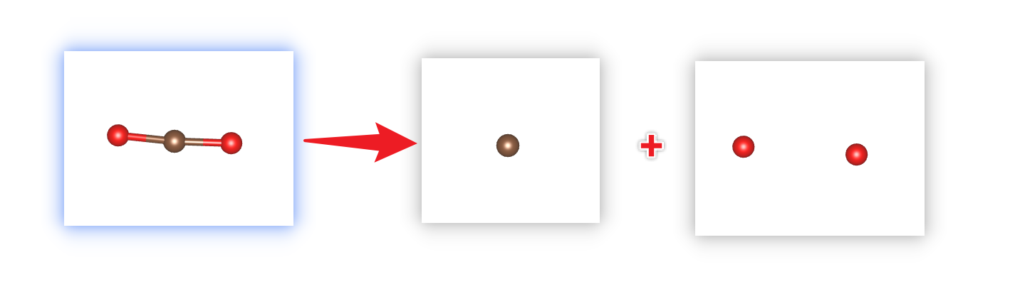
- Split the POSCAR
Let take the CO2 structure as the example again. Here we will take the C atom out to see what the operation does.
The C atom index is 1, so we should run rsgrad pos POSCAR -s -i 1
$ rsgrad pos POSCAR -s -i 1
[2022-07-14T15:49:32Z INFO  rsgrad::commands::pos] Reading POSCAR file "POSCAR" ...
[2022-07-14T15:49:32Z INFO  rsgrad::commands::pos] Splitting it to "POSCAR_A" and "POSCAR_B" ...
[2022-07-14T15:49:32Z INFO  rsgrad::commands::pos] "POSCAR_A" contains
[2022-07-14T15:49:32Z INFO  rsgrad::commands::pos]       C     1
[2022-07-14T15:49:32Z INFO  rsgrad::commands::pos] "POSCAR_B" contains
[2022-07-14T15:49:32Z INFO  rsgrad::commands::pos]       O     2
[2022-07-14T15:49:32Z INFO  rsgrad::commands::pos] "POSCAR_A" written
[2022-07-14T15:49:32Z INFO  rsgrad::commands::pos] "POSCAR_B" written
[2022-07-14T15:49:32Z INFO  rsgrad] Time used: 2.11275ms
The separated files should be like
$ bat POSCAR_A POSCAR_B
───────┬──────────────────────────────────────────────────────────────────────────
       │ File: POSCAR_A
───────┼──────────────────────────────────────────────────────────────────────────
   1   │ Generated by rsgrad, POSCAR with selected atoms
   2   │  1.0000000
   3   │       20.000000000       0.000000000       0.000000000
   4   │        0.000000000      20.000000000       0.000000000
   5   │        0.000000000       0.000000000      20.000000000
   6   │       C
   7   │       1
   8   │ Direct
   9   │       0.5000000000      0.5000000000     -0.5000000000 !      C-001    1
───────┴──────────────────────────────────────────────────────────────────────────
───────┬──────────────────────────────────────────────────────────────────────────
       │ File: POSCAR_B
───────┼──────────────────────────────────────────────────────────────────────────
   1   │ Generated by rsgrad, POSCAR complement
   2   │  1.0000000
   3   │       20.000000000       0.000000000       0.000000000
   4   │        0.000000000      20.000000000       0.000000000
   5   │        0.000000000       0.000000000      20.000000000
   6   │       O
   7   │       2
   8   │ Direct
   9   │       0.5754584708      0.4974961803      0.5000000000 !      O-001    1
  10   │       0.4249089652      0.5078477016      0.5000000000 !      O-002    2
───────┴──────────────────────────────────────────────────────────────────────────
The process schema:
Pseudo Potential
This command generates POTCAR according to POSCAR. The usage is simple: rsgrad pot in the directory with POSCAR presents.
To use this command, a configuration file is required like:
[functional-path]
PAW_PBE = "<path of PAW_PBE>"
PAW_LDA = "<path of PAW_LDA>"
and you need to put it at ~/.rsgrad for Linux/macOS,
and C:\Users\<YourUserName>\.rsgrad.toml for Windows.
Note: rsgrad pot will give some hint if you have no idea on how to write the file.
Then you can specify the element type in POSCAR, for example:
Cd2 S2 HSE optimized
   1.00000000000000
     4.1704589747753724    0.0000000049514629    0.0000000000000000
    -2.0852299788115007    3.6117232476351271   -0.0000000000000000
     0.0000000000000000   -0.0000000000000000    6.7822968954189937
   Cd   S
     2     2
Direct
  0.6666669999999968  0.3333330000000032  0.5001535716160643
  0.3333330000000032  0.6666669999999968  0.0001535716160644
  0.6666669999999968  0.3333330000000032  0.8768464283839381
  0.3333330000000032  0.6666669999999968  0.3768464283839381
Finally rsgrad-pot will read the line " Cd S ", and find the corresponding POTCAR and merge them.
In some cases, several elements does not have "standard" POTCAR that without suffix. E.g. the K/POTCAR
is not available for PBE functional. We provide two solutions for it:
- Write
K_svor other available K-related functionals in POSCARCd2 S2 HSE optimized 1.00000000000000 4.1704589747753724 0.0000000049514629 0.0000000000000000 -2.0852299788115007 3.6117232476351271 -0.0000000000000000 0.0000000000000000 -0.0000000000000000 6.7822968954189937 Cd K_sv 2 2 Direct 0.6666669999999968 0.3333330000000032 0.5001535716160643 ... - Use
aliasesfield in.rsgrad.toml
or[functional-path] ... aliases = { K = "K_sv" }[functional-path] ... [functional-path.aliases] K = "K_sv"
Help Message
rsgrad-pot
Generate the POTCAR according to POSCAR

USAGE:
    rsgrad pot [OPTIONS] [FUNCTIONAL]

ARGS:
    <FUNCTIONAL>
            Specify the functional type, now only "PAW_PBE"(or "paw_pbe") and "PAW_LDA"(or
            "paw_lda") are available

            [default: PAW_PBE]

OPTIONS:
    -c, --config <CONFIG>
            Specify the configuration file, if left blank, rsgrad will read `.rsgrad.toml` at your
            home dir

    -h, --help
            Print help information

    -p, --poscar <POSCAR>
            Specify the POSCAR file

            Note: the elements symbols' line should involve the specified valence configuration if
            you need. For example, if you need a `K_sv` POTCAR for `K`, just write `K_sv` in the
            POSCAR

            [default: ./POSCAR]

    -s, --save-in <SAVE_IN>
            Specify where the `POTCAR` would be written

            [default: ./]
Example
$ rsgrad pot
[2023-10-20T16:19:48Z INFO  rsgrad::settings] Reading rsgrad settings from "/Users/ionizing/.rsgrad.toml" ...
[2023-10-20T16:19:48Z INFO  rsgrad::settings] Checking rsgrad setting availability ...
[2023-10-20T16:19:48Z INFO  rsgrad::commands::pot] Reading POSCAR file "../tests/POSCAR.CdS_HSE" ...
[2023-10-20T16:19:48Z INFO  rsgrad::vasp_parsers::potcar] Reading POTCAR from "/Users/ionizing/apps/vasp/pp/potpaw_PBE.54/Cd/POTCAR"
[2023-10-20T16:19:48Z INFO  rsgrad::vasp_parsers::potcar] Reading POTCAR from "/Users/ionizing/apps/vasp/pp/potpaw_PBE.54/S/POTCAR"
[2023-10-20T16:19:48Z INFO  rsgrad::commands::pot] Writing POTCAR to "./POTCAR" ...
[2023-10-20T16:19:48Z INFO  rsgrad] Time used: 5.524643ms
Transition Dipole Moment
This command (rsgrad tdm) calculates the transition dipole moment(tdm)
between given bands, and then plot the peaks with plotly.
Note: This command can only calculate the TDM between bands in same k-point. The inter-kpoint transition is not supported yet. Also, this commands calculates the TDM in reciprocal space by
\[ TDM_{i\to j} = \langle \phi_j | e\cdot\vec{r} | \phi_i \rangle = e\cdot\frac{i\hbar}{m_e\Delta E_{ij}} \langle \phi_j | \vec{p} | \phi_i \rangle \]
Also, this command only calculates the TDM if \(j > i\), otherwise it will ignore the invalid \(i\to j\) pairs.
Help Message
$ rsgrad tdm --help
rsgrad-tdm
Calculate Transition Dipole Moment (TDM) between given bands.

Note: This command can only calculate the TDM between bands in same k-point. The inter-kpoint
transition is not supported yet. Also, this commands calculates the TDM in reciprocal space by

tdm_{i->j} = <phi_j|e*r|phi_i> = i*ħ/(ΔE*m)*<phi_j|p|phi_i>

USAGE:
    rsgrad tdm [OPTIONS] --ibands <IBANDS>... --jbands <JBANDS>...

OPTIONS:
        --barwidth <BARWIDTH>
            Specify the width of bars in the center of peaks. (eV)

            [default: 0.1]

        --gamma-half <GAMMA_HALF>
            Gamma Half direction of WAVECAR. You need to set this to 'x' or 'z' when processing
            WAVECAR produced by `vasp_gam`

            [possible values: x, z]

    -h, --help
            Print help information

        --htmlout <HTMLOUT>
            Write the plot of TDM to html file

            [default: tdm_smeared.html]

    -i, --ibands <IBANDS>...
            Initial band indices, start from 1

    -j, --jbands <JBANDS>...
            Final band indices, starts from 1

    -k, --ikpoint <IKPOINT>
            K-point index, starts from 1

            [default: 1]

        --npoints <NPOINTS>
            How many points in the x axis PER eV

            [default: 500]

        --peakout <PEAKOUT>
            Write the TDM peaks to raw txt file

            [default: tdm_peaks.txt]

    -s, --ispin <ISPIN>
            Spin index, 1 for up, 2 for down

            [default: 1]
            [possible values: 1, 2]

        --show
            Open the default browser to show the plot

        --sigma <SIGMA>
            Smearing width, in eV

            [default: 0.05]

        --to-inline-html
            Print the inline HTML to stdout

        --txtout <TXTOUT>
            Write the summed and smeared TDM to raw txt file

            [default: tdm_smeared.txt]

    -v, --verbose
            Print the calculated TDM to screen

    -w, --wavecar <WAVECAR>
            WAVECAR file path

            [default: ./WAVECAR]

        --xmax <XMAX>
            Highest energy scale for tdm_smeared.txt, default for max(dE) + 2.0

        --xmin <XMIN>
            Lowest energy scale for tdm_smeared.txt, default for min(dE) - 2.0
Example
The -i and -j arguments are required, or it will complain with error.
$ rsgrad tdm -i 2 -j {3..5}
[2022-08-10T07:26:46Z INFO  rsgrad::commands::tdm] Reading "./WAVECAR"
[2022-08-10T07:26:46Z INFO  rsgrad::commands::tdm] Writing peaks info to "tdm_peaks.txt" ...
[2022-08-10T07:26:46Z INFO  rsgrad::commands::tdm] Writing smeared TDM data to "tdm_smeared.txt"
[2022-08-10T07:26:46Z INFO  rsgrad::commands::tdm] Writing plot to "tdm_smeared.html"
[2022-08-10T07:26:46Z INFO  rsgrad] Time used: 56.655387ms
It produces the HTML like:
You can view the \(x\), \(y\) and \(z\) components of each peak by hovering on the thin bars at the center of peaks.
Note: If two peaks are in the same x position, one of them will be covered.
Then the tdm_peaks.txt should be like:
# iband jband     E_i     E_j      ΔE        Tx       Ty       Tz
      2     3  -5.974  -3.675   2.298     1.311    2.556    0.000
      2     4  -5.974  -3.675   2.298     2.556    1.311    0.000
      2     5  -5.974  -0.975   4.999     0.000    0.000    5.309
And the tdm_smeared.txt should be like:
# E(eV)    Tx(Debye)   Ty(Debye)   Tz(Debye)
         0.298325         0.007692         0.007692         0.001912         0.017295
         0.300240         0.007706         0.007706         0.001914         0.017326
         0.302155         0.007721         0.007721         0.001915         0.017357
         0.304070         0.007736         0.007736         0.001917         0.017389
         0.305985         0.007751         0.007751         0.001918         0.017420
         0.307900         0.007766         0.007766         0.001920         0.017451
...
...
Then you can plot the TDM peaks with other tools like OriginPro.
If your WAVECAR is produced by vasp_gam, you'd better specify the gamma half direction by --gamma-half x or --gamma-half z,
or rsgrad tdm will produce wrong results.
Gap
This command (rsgrad gap) calculates the band gap and prints positions of VBM and CBM.
There are two ways to run this command:
- Use
WAVECARonly. All required information can be extracted fromWAVECAR. - Or use
PROCARandOUTCARinstead.PROCARis read for the band energies, band occupations and k-point coordinates;OUTCARis read for the Fermi level only.
Note: Usually it's faster to parse results from WAVECAR.
If your system is a non-SCF calculation for band structure, you may need to specify the correct Fermi level by
rsgrad gap -e <put the correct E-fermi here>, the correct Fermi level can be obtained from the OUTCAR of SCF calculation.
Help Message
$ rsgrad gap --help
rsgrad-gap
Find band gap and print positions of VBM and CBM

USAGE:
    rsgrad gap [OPTIONS]

OPTIONS:
    -e, --efermi <EFERMI>      Specify Fermi level, if left empty, this value would be read from
                               WAVECAR or OUTCAR
    -h, --help                 Print help information
    -o, --outcar <OUTCAR>      OUTCAR file name, this file is parsed to get Fermi level only
                               [default: OUTCAR]
    -p, --procar <PROCAR>      PROCAR file name, OUTCAR is also needed to get Fermi level [default:
                               PROCAR]
    -w, --wavecar <WAVECAR>    WAVECAR file name, no more files needed [default: WAVECAR]
Example
- For metal system:
[2022-12-01T11:30:49Z INFO  rsgrad::commands::gap] Trying to parse "WAVECAR" ...
----------------------------------------
 Current system is         Metal
----------------------------------------
[2022-12-01T11:30:49Z INFO  rsgrad] Time used: 166.251241ms
- For non-spin-polarized direct gap system:
[2022-12-01T11:37:15Z INFO  rsgrad::commands::gap] Trying to parse "WAVECAR" ...
--------------------------------------------------------------------------------
 Current system has    Direct Gap    of   0.328    eV
  CBM @ k-point     1 of ( 0.000, 0.000, 0.000) , band   819 of    0.322 eV
  VBM @ k-point     1 of ( 0.000, 0.000, 0.000) , band   818 of   -0.006 eV
--------------------------------------------------------------------------------
[2022-12-01T11:37:15Z INFO  rsgrad] Time used: 253.556682ms
- For spin-polarized direct gap system:
$ rsgrad gap
[2022-12-01T11:38:16Z INFO  rsgrad::commands::gap] Trying to parse "WAVECAR" ...
--------------------------------------------------------------------------------
    ====================  Gap Info For     SPIN UP      ====================
 Current system has    Direct Gap    of   0.976    eV
  CBM @ k-point     1 of ( 0.000, 0.000, 0.000) , band   129 of    0.498 eV
  VBM @ k-point     1 of ( 0.000, 0.000, 0.000) , band   128 of   -0.478 eV
    ====================  Gap Info For    SPIN DOWN     ====================
 Current system has    Direct Gap    of   0.980    eV
  CBM @ k-point     1 of ( 0.000, 0.000, 0.000) , band   129 of    0.499 eV
  VBM @ k-point     1 of ( 0.000, 0.000, 0.000) , band   128 of   -0.481 eV
--------------------------------------------------------------------------------
[2022-12-01T11:38:16Z INFO  rsgrad] Time used: 31.744371ms
- For non-spin-polarized indirect gap system:
$ rsgrad gap
[2022-12-01T11:40:52Z INFO  rsgrad::commands::gap] Trying to parse "WAVECAR" ...
--------------------------------------------------------------------------------
 Current system has   Indirect Gap   of   1.160    eV
  CBM @ k-point    25 of ( 0.000, 0.444, 0.444) , band     5 of    1.097 eV
  VBM @ k-point    17 of ( 0.000, 0.000, 0.000) , band     4 of   -0.062 eV
--------------------------------------------------------------------------------
[2022-12-01T11:40:52Z INFO  rsgrad] Time used: 22.565948ms
UnitConversion
This command (rsgrad uc) converts input quantity to units representing same energy.
Metric prefixes are supported, from Atto(a, 10-18) to Exa(E, 1018).
Here are supported prefixes and corresponding acronyms:
| Metric prefix | Acronym | Base 10 |
|---|---|---|
| atto | a | 10-18 |
| femto | f | 10-15 |
| pico | p | 10-12 |
| nano | n | 10-9 |
| micro | μ | 10-6 |
| milli | m | 10-3 |
| -- | -- | 100 |
| Kilo | K | 103 |
| Mega | M | 106 |
| Giga | G | 109 |
| Tera | T | 1012 |
| Peta | P | 1015 |
| exa | E | 1018 |
If you use acronyms, note that prefixes smaller than 1 (from a, atto to m, micro) must be lowercased whereas the prefixes lager than 1 (from K, Kilo to E, Exa) must be uppercased.
Supported units:
| Unit | Symbol |
|---|---|
| Hartree | Ha |
| Wavenumber | cm-1 |
| Temperature(Kelvin) | K |
| Calorie per mole | Cal/mol |
| Joule per mole | J/mol |
| Wavelength | m |
| Period | s |
| Electron volt | eV |
| Frequency | Hz |
Help Message
$ rsgrad uc
Conversion between various energy units

Usage: rsgrad uc [INPUT]...

Arguments:
  [INPUT]...  Input energy quantity to be converted. Multiple input are supported

Options:
  -h, --help  Print help

Try `rsgrad uc 298K` to see what happens.
Examples
$ rsgrad uc 298K
==================== Processing input "298K" ====================
  298.000000 K ==   943.709369 μHa
  298.000000 K ==   207.125149 cm-1
  298.000000 K ==   298.000000 K
  298.000000 K ==   592.202785 Cal/mol
  298.000000 K ==     2.477776 KJ/mol
  298.000000 K ==    48.281101 μm
  298.000000 K ==   161.048425 fs
  298.000000 K ==    25.679653 meV
  298.000000 K ==     6.209312 THz
================================================================================

[2024-09-11T07:21:07Z INFO  rsgrad] Time used: 470.398µs
You can also input multiple quantities at a time
$ rsgrad uc 298K 25meV 300THz
==================== Processing input "298K" ====================
  298.000000 K ==   161.048425 fs
  298.000000 K ==   207.125149 cm-1
  298.000000 K ==     2.477776 KJ/mol
  298.000000 K ==    25.679653 meV
  298.000000 K ==    48.281101 μm
  298.000000 K ==   943.709369 μHa
  298.000000 K ==   592.202785 Cal/mol
  298.000000 K ==     6.209312 THz
  298.000000 K ==   298.000000 K
================================================================================

==================== Processing input "25meV" ====================
   25.000000 meV ==   165.426708 fs
   25.000000 meV ==   201.643250 cm-1
   25.000000 meV ==     2.412198 KJ/mol
   25.000000 meV ==    25.000000 meV
   25.000000 meV ==    49.593677 μm
   25.000000 meV ==   918.732590 μHa
   25.000000 meV ==   576.529191 Cal/mol
   25.000000 meV ==     6.044973 THz
   25.000000 meV ==   290.112953 K
================================================================================

==================== Processing input "300THz" ====================
  300.000000 THz ==     3.333333 fs
  300.000000 THz ==    10.007154 Kcm-1
  300.000000 THz ==   119.712599 KJ/mol
  300.000000 THz ==     1.240700 eV
  300.000000 THz ==   999.308150 nm
  300.000000 THz ==    45.594872 mHa
  300.000000 THz ==    28.611998 KCal/mol
  300.000000 THz ==   300.000000 THz
  300.000000 THz ==    14.397729 KK
================================================================================

[2024-09-11T07:27:53Z INFO  rsgrad] Time used: 544.171µs
Model Non-adiabatic Coupling
This command (rsgrad model-nac) calculates the model non-adiabatic coupling
for NAMD-LMI (a subset of Hefei-NAMD).
NOTE: This command calculates momentum matrix element <i|p|j> using velocity gauge only,
thus the transition dipole moment in length gauge <i|r|j> is not used.
Help Message
$ rsgrad model-nac --help
Calculate model non-adiabatic coupling (NAC) for NAMD-LMI (a subset of Hefei-NAMD).

This NAC contains eigenvalues and transition dipole moment (TDM) calculated from selected WAVECAR. The phonon contribution is wipped out, which means the eigenvalues and TDM stay staic over the time, and the NAC (<i|d/dt|j>) vanishes.

Detailed fields of the produced file:
 - ikpoint: K point index, counts from 1;
 - nspin: number of spin channels;
 - nbands: Number of total bands in WAVECAR;
 - brange: selected band indices, <start> ..= <end>, index counts from 1;
 - nbrange: number of selected bands, nbrange = end - start + 1;
 - efermi: Fermi's level;
 - potim: ionic time step;
 - temperature: 1E-6 Kelvin as default;
 - eigs: band eigenvalues;
 - pij_r/pij_i: real and imaginary part of <i|p|j>;
 - proj: Projection on each orbitals of selected bands, cropped from PROCAR.

Some fields not listed here are not meaningful but essential for the NAMD-LMI.

Usage: rsgrad model-nac [OPTIONS]

Options:
  -w, --wavecar <WAVECAR>
          WAVECAR file name

          [default: ./WAVECAR]

      --gamma-half <GAMMA_HALF>
          Gamma Half direction of WAVECAR. You need to set this to 'x' or 'z' when processing WAVECAR produced by `vasp_gam`

          [possible values: x, z]

  -k, --ikpoint <IKPOINT>
          One selected K-Point index, count starts from 1.

          Example: --ikpoint 2

          [default: 1]

      --brange <BRANGE> <BRANGE>
          Selected band range, starts from 1.

          Example: --brange 24 42

      --potim <POTIM>
          Ionic time step in femtosecond (fs)

          [default: 1]

  -p, --procar <PROCAR>
          PROCAR file name for band projection parsing

          [default: ./PROCAR]

  -o, --h5out <H5OUT>
          Output file name

          [default: ./NAC-0K.h5]

  -h, --help
          Print help (see a summary with '-h')
Example
The --brange <start> <end> is required, or it will complain with error.
rsgrad model-nac --brange 107 110
[2024-11-18T04:17:11Z INFO  rsgrad::commands::modelnac] Reading WAVECAR: "./WAVECAR"
[2024-11-18T04:17:11Z INFO  rsgrad::commands::modelnac] Reading PROCAR: "./PROCAR"
[2024-11-18T04:17:11Z INFO  rsgrad::commands::modelnac] Saving to "./NAC-0K.h5"
[2024-11-18T04:17:11Z INFO  rsgrad] Time used: 87.687584ms
NormalCAR
rsgrad normalcar writes PAW projector coefficients from WAVECAR, POSCAR, and POTCAR.
The generated NormalCAR is useful for workflows that need the projector coefficients
β = ⟨p̃_i|ψ̃⟩, such as spin-orbit and other PAW-based post-processing.
Help Message
$ rsgrad normalcar --help
Write NormalCAR (PAW projector coefficients) from POSCAR + POTCAR + WAVECAR.

The NormalCAR stores the PAW projector coefficients β = ⟨p̃_i|ψ̃⟩ for every spin/k-point/band, useful for spinorb and other post-processing tools.

Usage: rsgrad normalcar [OPTIONS]

Options:
      --wavecar <WAVECAR>
          WAVECAR file path

          [default: WAVECAR]

      --poscar <POSCAR>
          POSCAR file path

          [default: POSCAR]

      --potcar <POTCAR>
          POTCAR file path

          [default: POTCAR]

  -o, --output <OUTPUT>
          Output file path. If extension is .npz, write numpy npz format; otherwise write binary NormalCAR

          [default: NormalCAR]

  -h, --help
          Print help (see a summary with '-h')
Examples
Write the binary NormalCAR used by VASP-style post-processing:
$ rsgrad normalcar --wavecar WAVECAR --poscar POSCAR --potcar POTCAR -o NormalCAR
Write the same coefficients as a NumPy archive:
$ rsgrad normalcar --wavecar WAVECAR --poscar POSCAR --potcar POTCAR -o cproj.npz
If the output file ends with .npz, rsgrad writes a NumPy-friendly archive. Otherwise it writes
the binary NormalCAR format.
Overlap
rsgrad overlap computes wavefunction overlaps between two WAVECAR files.
By default it includes the PAW one-centre correction and evaluates the all-electron overlap
S_{ij}(k) = <Φ_i^a(k)|Φ_j^b(k)>.
If you only want the pseudo-wavefunction overlap, use --pseudo.
Help Message
$ rsgrad overlap --help
Compute AE wavefunction overlaps between two WAVECARs.

Computes S_{ij}(k) = <Φ_i^a(k)|Φ_j^b(k)> including the PAW one-centre correction.

Usage: rsgrad overlap [OPTIONS] --wavecar2 <WAVECAR2> --poscar2 <POSCAR2> --ibands <IBANDS>... --jbands <JBANDS>...

Options:
      --wavecar1 <WAVECAR1>
          First WAVECAR file path

          [default: WAVECAR]

      --wavecar2 <WAVECAR2>
          Second WAVECAR file path (required)

      --poscar1 <POSCAR1>
          First POSCAR file path

          [default: POSCAR]

      --poscar2 <POSCAR2>
          Second POSCAR file path (required)

      --potcar <POTCAR>
          POTCAR file path (shared between both structures)

          [default: POTCAR]

      --ispins <ISPINS>...
          Spin indices (1-indexed). Multiple values allowed

          [default: 1]

      --kpoints <KPOINTS>...
          K-point indices (1-indexed). Multiple values allowed

          [default: 1]

      --ibands <IBANDS>...
          Initial band index specs (e.g. "1:10" "15" "1:20:2"). 1-indexed

      --jbands <JBANDS>...
          Final band index specs (e.g. "1:10" "15" "1:20:2"). 1-indexed

      --pseudo
          If set, skip the PAW one-centre correction (pseudo-only overlap)

  -o, --output <OUTPUT>
          Output file path. Extension determines format: .npz → numpy, else text table

          [default: overlap.dat]

  -h, --help
          Print help (see a summary with '-h')
Examples
Compute overlaps between two calculations and write a text table:
$ rsgrad overlap \
    --wavecar1 WAVECAR \
    --wavecar2 ../other/WAVECAR \
    --poscar1 POSCAR \
    --poscar2 ../other/POSCAR \
    --potcar POTCAR \
    --ibands 1:10 \
    --jbands 1:10 \
    -o overlap.dat
Write the overlap data as a NumPy archive:
$ rsgrad overlap \
    --wavecar2 ../other/WAVECAR \
    --poscar2 ../other/POSCAR \
    --ibands 1:20 \
    --jbands 1:20 \
    -o overlap.npz
Use --pseudo if you want pseudo-only overlaps without the PAW correction:
$ rsgrad overlap --wavecar2 ../other/WAVECAR --poscar2 ../other/POSCAR --ibands 1:10 --jbands 1:10 --pseudo
Feedback
We are happy that you reach here. As an open-source project, rsgrad welcomes feedback.
-
If you have want to add features to
rsgrad, just open an issue at GitHub Issues. We also created a feature-requests list, you can follow it at this page. -
If
rsgradcomplains something or produces wrong result, just open an issue at GitHub Issues. We are grateful if you can provide the input files in order that we can reproduce the issue conveniently, thus solve the issue as soon as possible. -
If you are interested in
rsgradand want to contribute to the source code, just forkrsgradand create pull requests at Pull Requests. We are super grateful if you can contribute torsgrad.