Introduction

NAMD-LMI is a subset of Hefei-NAMD with light-matter interaction (LMI) support.

Hefei-NAMD is an ab initio non-adiabatic molecular dynamics program to investigate the ultrafast excited carrier dynamics in real and momentum space, energy and time scale.

Now NAMD-LMI is capable to

• Study carrier dynamics in real space and energy relaxation without laser field at finite temperture;
• Study photo-excitaion process and stimulated emission process and carrier dynamics in the laser field at zero temperature;
• Study carrier dynamics both under the perturbation of phonon and LMI.

You may need watch the former tutorials to learn the basic concept and procedures of Hefei-NAMD in the following pages:

• Basic Hefei-NAMD
• Hefei-NAMD with CA-NAC
• Hefei-NAMD with excitonic effects

Installation

There are two ways to install NAMD-LMI, downloading the pre-built binaries or building from scratch.

Download the binary from Github Release

We provide the pre-built binaries at Github Release.

There are several platforms we support with pre-built binaries, in which we can identify them by their file names parts:

• namd_lmi-: the version of NAMD-LMI;
• linux/macos/windows: which operating system it runs on;
• x86_64/aarch64: which CPU architecture it runs on;
• mkl-system/mkl-static/openblas-system/openblas-static: which BLAS implementation and which link scheme, where xxx-system requires you install corresponding BLAS implementation on system, while xxx-static statically link against to BLAS (which means you needn't install anything else) but come with larger binary sizes.
• .tar.gz/zip: which compressor format it uses. You need to decompress the binary first.

Example:

• namd_lmi-1.0.0-linux-x86_64-mkl-system.tar.gz should run on an x86 machine with 64-bit Linux installed, where the Intel-MKL should be installed.
• namd_lmi-1.0.0-macos-x86_64-mkl-system.tar.gz should run on macOS with Intel chip.
• namd_lmi-1.0.0-macos-aarch64-mkl-system.tar.gz should run on macOS with Apple Silicon.
• namd_lmi-1.0.0-windows-x86_64-mkl-static.zip should run on Windows 7 or upper with Intel/AMD or other x86 chips.

Build from scratch

The build requires Internet accessibility and Rust toolchain, Intel-MKL libraries.

• If you haven't installed Rust toolchain, run curl --proto '=https' --tlsv1.2 -sSf https://sh.rustup.rs | sh and follow the instructions to configure it. When you finished the toolchain installation, you should be able to run cargo in command-line. Detailed instructions can be found here.
• If you have installed Rust toolchain and Intel-MKL already, just run cargo install --git https://github.com/Ionizing/NAMD-LMI. Several minutes later, the namd_lmi binary should be installed to ~/.cargo/bin, no need to modify the $PATH (or %PATH% on Windows).

There are four features to link BLAS implementations:

• intel-mkl-system: dynamically link against pre-installed Intel-MKL library. You need to install Intel-MKL first.
• intel-mkl-static: statically link against Intel-MKL library. If no pre-installed MKL is found, it will download Intel-MKL 2020 from web by itself.
• openblas-system: dynamically link against pre-installed OpenBLAS. You need to install OpenBLAS first.
• openblas-static: statically link against OpenBLAS library. If no pre-installed OpenBLAS is found, it will download OpenBLAS source code and build it from scratch.

Test the installation

Once you obtain the namd_lmi binary, just put it in your PATH, and then you should be able to run it with the output like

$ namd_lmi
+----------------------------------------------------------------------+
|                                                                      |
|    _   _            __  __  _____           _       __  __  _____    |
|   | \ | |    /\    |  \/  ||  __ \         | |     |  \/  ||_   _|   |
|   |  \| |   /  \   | \  / || |  | | ______ | |     | \  / |  | |     |
|   | . ` |  / /\ \  | |\/| || |  | ||______|| |     | |\/| |  | |     |
|   | |\  | / ____ \ | |  | || |__| |        | |____ | |  | | _| |_    |
|   |_| \_|/_/    \_\|_|  |_||_____/         |______||_|  |_||_____|   |
|                                                                      |
+----------------------------------------------------------------------+

Welcome to use namd!
    current version:    0.1.0
    git hash:           d659586
    author(s):          Ionizing
    host:               x86_64-unknown-linux-gnu
    built time:         2024-11-19 15:34:05 +08:00


Usage: namd_lmi <COMMAND>

Commands:
  nac      Calculate non-adiabatic coupling (NAC) including `<j| d/dt |k>` and momentum matrix `<i| p |j>`
  hamil    Generate the Hamiltonian from NAC according to config file
  surfhop  Perform the surface-hopping process with given Hamiltonian file and config file
  help     Print this message or the help of the given subcommand(s)

Options:
  -h, --help     Print help (see more with '--help')
  -V, --version  Print version

Overall process

NAMD-LMI is divided into three parts: nac, hamil and surfhop, corresponding to the calculation of non-adiabatic coupling, Hamiltonian and surface hopping.

1. Run VASP like traditional Hefei-NAMD;
2. Run namd_lmi nac -c config to calculate non-adiabatic coupling. A visualization script nac_plot.py is also available via namd_lmi nac --generate pp.
3. Run namd_lmi hamil -c config to generate Hamiltonian plus external field. The external field is described in a rhai script, which can be generated via namd_lmi hamil --generate efield. A visualization script hamil_plot.py is also available via namd_lmi hamil --generate pp.
4. Run namd_lmi surfhop -c config to run surface hopping and get the real time evolution of the population. A visualization script surfhop_plot.py is also available via namd_lmi surfhop --generate pp.

Non-adiabatic Coupling

In Hefei-NAMD non-adiabatic coupling (NAC) is defined as the derivative of wavefunctions

\begin{equation} \mathbf{D}_{jk} = \mel{\phi_j}{\dv{t}}{\phi_k} \end{equation}

where $\phi$ is the Kohn-Sham (KS) orbitals calculated by VASP.

To simulate photo-excitations process, momentum matrix element \(\mathbf{P}_{jk} = \mel{j}{\mathbf{p}}{k}\) is needed to calculate the light-matter interaction (LMI) term

\begin{equation} \mathcal{H}_{jk}^{\mathrm{LMI}} = -e \frac{\mathbf{A}}{m_e} \mel{j}{\mathbf{p}}{k} \end{equation}

in which $\mathbf{p}$ is the momentum opeartor, and \(\mathbf{A}\) is the vector potential of external field.

NOTE: namd_lmi is capable of calculating both \(\mathbf{D}_{jk}\) and \(\mathbf{P}_{jk}\).

Help message

$ namd_lmi nac
Calculate non-adiabatic coupling (NAC) including `<j| d/dt |k>` and momentum matrix `<i| p |j>`

Usage: namd_lmi nac [OPTIONS]

Options:
  -n, --nthreads <NTHREADS>
          Number of threads for parallel calculation.

          If 0 is set, it will fall back to the number of logic CPU cores of you machine.

          [default: 0]

  -c, --config <CONFIG>
          Config file name.

          Aliases: "cfg", "conf".

          [default: nac_config.toml]

      --generate <GENERATE>
          Generate auxiliary files for the calculation and analysis.

          The calculation will not run if this flag is set.

          Alias: "gen"

          Possible values:
          - config-template:      Generate config template for NAC calculation. Aliases: "config", "cfg", "conf"
          - postprocess-template: Generate post-process scripts for NAC analysis. Aliases: "post-process", "postprocess", "pp"

  -h, --help
          Print help (see a summary with '-h')

Procedures

1. Generate a configuration template.

   $ namd_lmi nac --generate conf
   2024-11-19 20:26:10 [ INFO] Global logger initialized with targets being stderr and "./globalrun.log"
   2024-11-19 20:26:10 [ INFO] Writing `01_nac_config_template.toml ...`
   2024-11-19 20:26:10 [ INFO] Time used: 1.351249ms
   

   where the 01_nac_config_template.toml reads

   		 rundir = "../run"
   		ikpoint = 1
   		 brange = [0, 0]
   			nsw = 2000
   		 ndigit = 4
   		  potim = 1
   	temperature = 0
   phasecorrection = true
   	   nacfname = "NAC.h5"
   

2. Modify the configuration according to your AIMD parameters.

   If you are familiar with the original Hefei-NAMD procedure, the parameters in 01_nac_config_template.toml is not hard to understand:

   • rundir string: AIMD directory where thousands of SCF with WAVECARs lies within.
   • ikpoint integer: Which K point to choose, the index counts from 1. For now, you can only choose one K point is selectable to calculate NAC and momentum matrix elements.
   • brange [integer, integer]: Selected band range for calculation. [100, 120] will select band from 100 to 120 to do the calculation, 21 bands in total.
   • nsw integer: Number of steps in AIMD. If there are 2000 steps in your run/, this field should be 2000.
   • ndigit integer: Number of digits for the index of each step. If the directories in your run/ are 00001 ... 02000, this field should be 5.
   • potim float: Time step of the AIMD, consistent with the POTIM in INCAR during NVE.
   • temperature float: Temperature of the MD, consistent with the TEEND in INCAR during NVT.
   • phasecorrection bool: Do phase correction for the KS orbitals or not. Should be either true or false. Usually this term is essential for the photo-excitation process.
   • nacfname string: Output file name.

   NOTE: The string fields must be surrounded with quotation mark "".

3. Do the coupling calculation.

   This process is quite simple

   $ namd_lmi nac -c 01_nac_config_template.toml
   2024-11-19 21:06:20 [ INFO] Global logger initialized with targets being stderr and "./globalrun.log"
   2024-11-19 21:06:20 [ INFO]
   +----------------------------------------------------------------------+
   |                                                                      |
   |    _   _            __  __  _____           _       __  __  _____    |
   |   | \ | |    /\    |  \/  ||  __ \         | |     |  \/  ||_   _|   |
   |   |  \| |   /  \   | \  / || |  | | ______ | |     | \  / |  | |     |
   |   | . ` |  / /\ \  | |\/| || |  | ||______|| |     | |\/| |  | |     |
   |   | |\  | / ____ \ | |  | || |__| |        | |____ | |  | | _| |_    |
   |   |_| \_|/_/    \_\|_|  |_||_____/         |______||_|  |_||_____|   |
   |                                                                      |
   +----------------------------------------------------------------------+
   
   Welcome to use namd!
       current version:    0.1.0
       git hash:           d659586
       author(s):          Ionizing
       host:               x86_64-unknown-linux-gnu
       built time:         2024-11-19 15:34:05 +08:00
   
   2024-11-19 21:06:20 [ INFO] Running with 0 threads.
   2024-11-19 21:06:20 [ INFO] Got NAC config:
   ####         NAMD-lmi config for Non-Adiabatic Coupling (NAC) calculation       ####
   ####    YOU NEED TO CHANGE THE PARAMETERS IN THE FOLLOWING TO FIT YOU SYSTEM    ####
   
                  rundir = "../../aimd/static_ncl_40/run/"
                 ikpoint = 1
                  brange = [213, 220]
                     nsw = 2000
                  ndigit = 4
                   potim = 1
             temperature = 300
         phasecorrection = true
                nacfname = "NAC.h5"
   
   2024-11-19 21:06:20 [ INFO] No pre-calculated NAC available, start calculating from scratch in "../../aimd/static_ncl_40/run/"/.../WAVECARs ...
   2024-11-19 21:06:20 [ INFO]  Calculating couplings between "../../aimd/static_ncl_40/run/0001" and "../../aimd/static_ncl_40/run/0002" ..., remains:   1999
   2024-11-19 21:06:20 [ INFO]  Calculating couplings between "../../aimd/static_ncl_40/run/0312" and "../../aimd/static_ncl_40/run/0313" ..., remains:   1998
   2024-11-19 21:06:20 [ INFO]  Calculating couplings between "../../aimd/static_ncl_40/run/1000" and "../../aimd/static_ncl_40/run/1001" ..., remains:   1997
   2024-11-19 21:06:20 [ INFO]  Calculating couplings between "../../aimd/static_ncl_40/run/0218" and "../../aimd/static_ncl_40/run/0219" ..., remains:   1996
   2024-11-19 21:06:20 [ INFO]  Calculating couplings between "../../aimd/static_ncl_40/run/0078" and "../../aimd/static_ncl_40/run/0079" ..., remains:   1995
   2024-11-19 21:06:20 [ INFO]  Calculating couplings between "../../aimd/static_ncl_40/run/0132" and "../../aimd/static_ncl_40/run/0133" ..., remains:   1994
   ...
   2024-11-19 21:08:31 [ INFO]  Calculating couplings between "../../aimd/static_ncl_40/run/1370" and "../../aimd/static_ncl_40/run/1371" ..., remains:      5
   2024-11-19 21:08:31 [ INFO]  Calculating couplings between "../../aimd/static_ncl_40/run/1358" and "../../aimd/static_ncl_40/run/1359" ..., remains:      4
   2024-11-19 21:08:31 [ INFO]  Calculating couplings between "../../aimd/static_ncl_40/run/1216" and "../../aimd/static_ncl_40/run/1217" ..., remains:      3
   2024-11-19 21:08:31 [ INFO]  Calculating couplings between "../../aimd/static_ncl_40/run/1217" and "../../aimd/static_ncl_40/run/1218" ..., remains:      2
   2024-11-19 21:08:31 [ INFO]  Calculating couplings between "../../aimd/static_ncl_40/run/1215" and "../../aimd/static_ncl_40/run/1216" ..., remains:      1
   2024-11-19 21:08:32 [ INFO] Time used: 72.490979406s
   

   namd_lmi nac uses rayon to utilize multi-threaded parallelism and you can specify the number of threads used by this command via -n/--nthreads. For example namd_lmi -c 01_nac_config_template.toml -n 32 uses 32 threads to calculate the couplings.

4. Visualize couplings

   Run namd_lmi nac --generate pp to get a Python script to visualize the produced NAC.h5

   $ namd_lmi nac --generate pp
   2024-11-19 21:14:22 [ INFO] Global logger initialized with targets being stderr and "./globalrun.log"
   2024-11-19 21:14:22 [ INFO] Writing `nac_plot.py` ...
   2024-11-19 21:14:22 [ INFO] Time used: 1.241002ms 
   
   $ python3 ./nac_plot.py
   Writing nac_bands.png
   Writing nac_nac.png
   

   And the produced .pngs should look like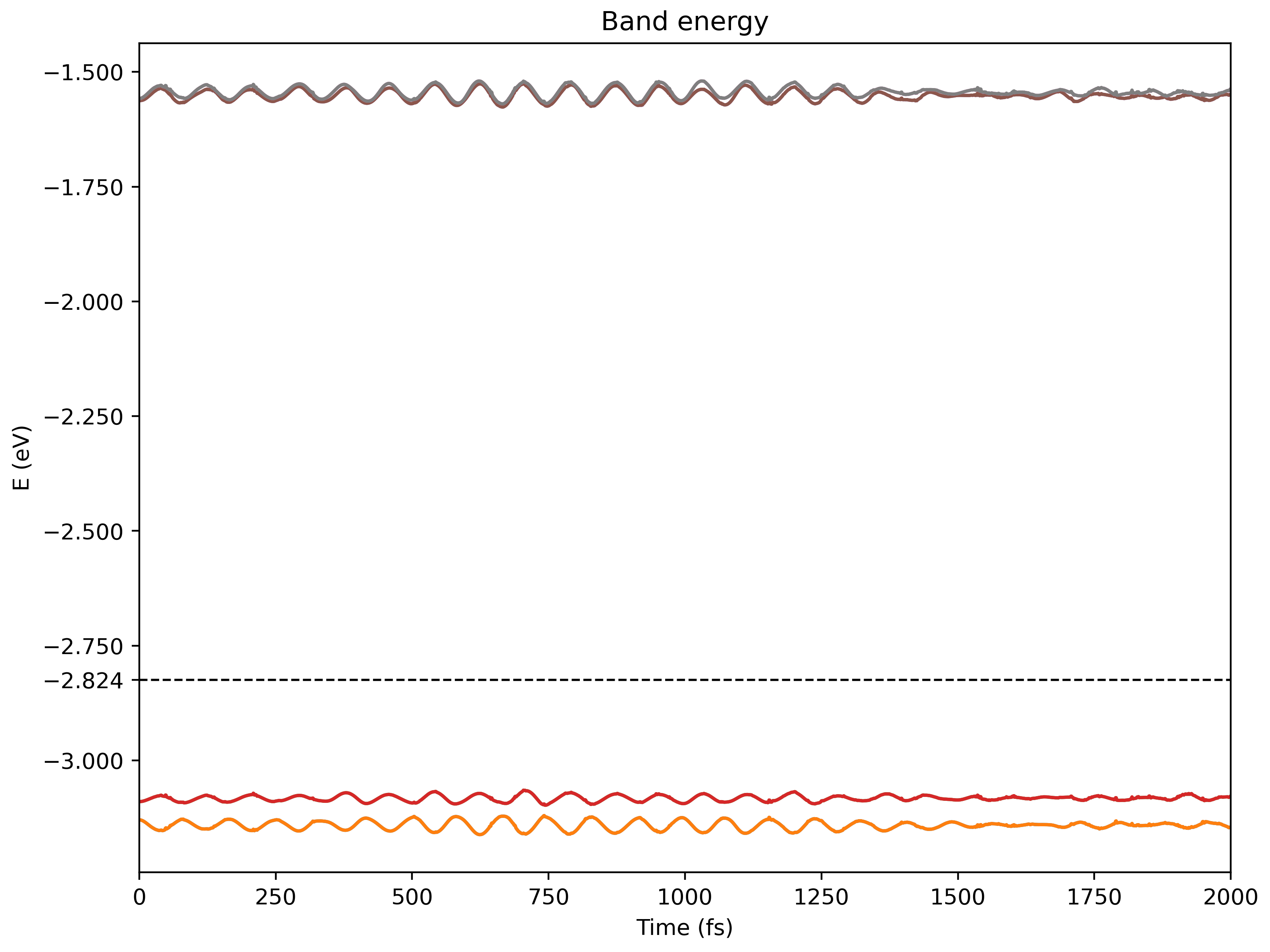

   

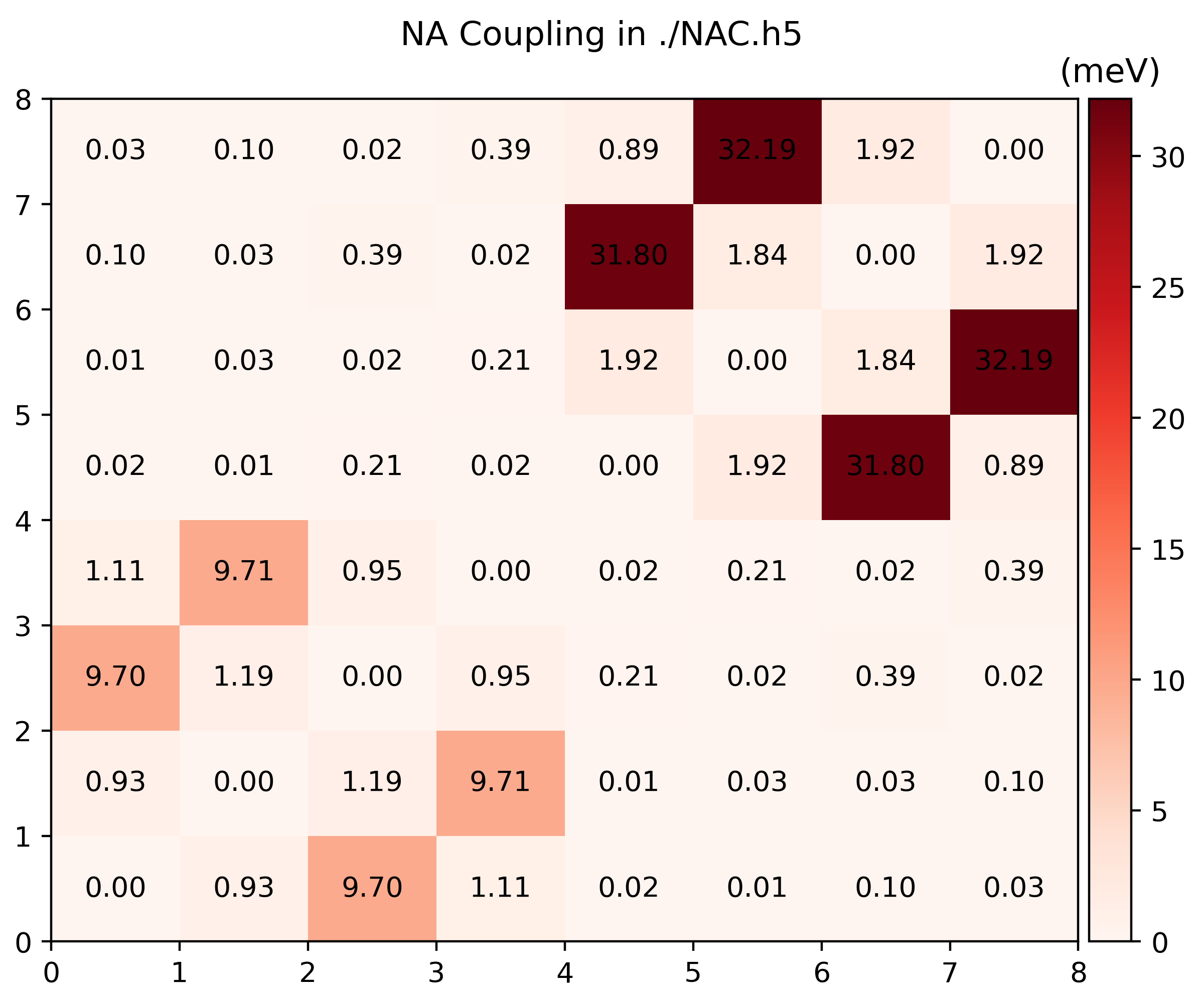
   You can modify nac_plot.py to visualize whatever you want.

Data fields of NAC.h5

$ h5dump -H NAC.h5
HDF5 "NAC.h5" {
GROUP "/" {
   DATASET "brange" {
      DATATYPE  H5T_ARRAY { [2] H5T_STD_U64LE }
      DATASPACE  SCALAR
   }
   DATASET "efermi" {
      DATATYPE  H5T_IEEE_F64LE
      DATASPACE  SCALAR
   }
   DATASET "eigs" {
      DATATYPE  H5T_IEEE_F64LE
      DATASPACE  SIMPLE { ( 1999, 1, 8 ) / ( 1999, 1, 8 ) }
   }
   DATASET "ikpoint" {
      DATATYPE  H5T_STD_U64LE
      DATASPACE  SCALAR
   }
   DATASET "nbands" {
      DATATYPE  H5T_STD_U64LE
      DATASPACE  SCALAR
   }
   DATASET "nbrange" {
      DATATYPE  H5T_STD_U64LE
      DATASPACE  SCALAR
   }
   DATASET "ndigit" {
      DATATYPE  H5T_STD_U64LE
      DATASPACE  SCALAR
   }
   DATASET "nspin" {
      DATATYPE  H5T_STD_U64LE
      DATASPACE  SCALAR
   }
   DATASET "nsw" {
      DATATYPE  H5T_STD_U64LE
      DATASPACE  SCALAR
   }
   DATASET "olaps_i" {
      DATATYPE  H5T_IEEE_F64LE
      DATASPACE  SIMPLE { ( 1999, 1, 8, 8 ) / ( 1999, 1, 8, 8 ) }
   }
   DATASET "olaps_r" {
      DATATYPE  H5T_IEEE_F64LE
      DATASPACE  SIMPLE { ( 1999, 1, 8, 8 ) / ( 1999, 1, 8, 8 ) }
   }
   DATASET "phasecorrection" {
      DATATYPE  H5T_ENUM {
         H5T_STD_I8LE;
         "FALSE"            0;
         "TRUE"             1;
      }
      DATASPACE  SCALAR
   }
   DATASET "pij_i" {
      DATATYPE  H5T_IEEE_F64LE
      DATASPACE  SIMPLE { ( 1999, 1, 3, 8, 8 ) / ( 1999, 1, 3, 8, 8 ) }
   }
   DATASET "pij_r" {
      DATATYPE  H5T_IEEE_F64LE
      DATASPACE  SIMPLE { ( 1999, 1, 3, 8, 8 ) / ( 1999, 1, 3, 8, 8 ) }
   }
   DATASET "potim" {
      DATATYPE  H5T_IEEE_F64LE
      DATASPACE  SCALAR
   }
   DATASET "proj" {             // This part is cropped from PROCARs
      DATATYPE  H5T_IEEE_F64LE
      DATASPACE  SIMPLE { ( 1999, 4, 8, 36, 9 ) / ( 1999, 4, 8, 36, 9 ) }
   }
   DATASET "temperature" {
      DATATYPE  H5T_IEEE_F64LE
      DATASPACE  SCALAR
   }
}
}

Hamiltonian

The Hamiltonian here is simply a cropped coupling of the Non-adiabatic couplings plus the external field.

The total Hamiltonian of namd_lmi consists of three parts: \begin{equation} \mathcal{H} = \mathcal{H}^0 + \mathcal{H}^{NAC} + \mathcal{H}^{LMI} \end{equation} where \(\mathcal{H}^0\) is just eigenvalues of KS orbitals and \(\mathcal{H}^{NAC}_{jk} = -i\hbar \mathbf{D}_{jk}\) models the e-ph and spin-orbit coupling (if LSORBIT=.TRUE. is used). The LMI term reads \(\mathcal{H}_{jk}^{\mathrm{LMI}} = -e \frac{\mathbf{A}}{m_e} \mel{j}{\mathbf{p}}{k}\). The vector potential term \(\mathbf{A}\) is calculated by integrating the external electric field \begin{equation} \mathbf{A}(t) = - \int_0^t \mathbf{E}(t') \dd t' \end{equation}

Help message

$ namd_lmi hamil --help
Generate the Hamiltonian from NAC according to config file

Usage: namd_lmi hamil [OPTIONS]

Options:
  -c, --config <CONFIG>
          Config file name.

          Aliases: "cfg", "conf".

          [default: hamil_config.toml]

      --generate <GENERATE>
          Generate auxiliary files for the calculation and analysis.

          The generation of Hamiltonian will not run if this flag is set.

          Alias: "gen".

          Possible values:
          - config-template:      Generate config template for Hamiltonian generation. Aliases: "config", "cfg" and "conf"
          - efield-template:      Generate script template for external electric field. Aliases: "efield", "ef"
          - postprocess-template: Generate post-process scripts for Hamiltonian analysis. Aliases: "post-process", "postprocess", "pp"

  -h, --help
          Print help (see a summary with '-h')

Procedures

1. Generate a configuration template, and an optical field description file

   $ namd_lmi hamil --generate conf
   2024-11-19 21:49:48 [ INFO] Global logger initialized with targets being stderr and "./globalrun.log"
   2024-11-19 21:49:48 [ INFO] Writing `02_hamil_config_template.toml` ...
   2024-11-19 21:49:48 [ INFO] Writing config to file "02_hamil_config_template.toml"
   2024-11-19 21:49:48 [ INFO] Time used: 1.624654ms
   
   $ namd_lmi hamil --generate efield
   2024-11-20 11:34:14 [ INFO] Global logger initialized with targets being stderr and "./globalrun.log"
   2024-11-20 11:34:14 [ INFO] Writing `efield_template.rhai` ...
   2024-11-20 11:34:14 [ INFO] Time used: 977.069µs
   

2. Modify the Hamiltonian configuration file and optical description file

   • Hamiltonian configuration

     The file 02_hamil_config.toml should read

     # NAMD-lmi config for Hamiltonian generation
     
           ikpoint = 1
        basis_list = "215..220"
      basis_labels = ["VBM-1", "VBM", "CBM", "CBM+1", "CBM+2", "CBM+3"]
         nac_fname = "NAC.h5"
      efield_fname = "./efield.rhai"
       hamil_fname = "HAMIL.h5"
        propmethod = "Expm"
           scissor = 1.5 # unit: eV
     

     Explanation of each field:

     • ikpoint integer: K point index, consistent with NAC's configuration.

     • basis_list string: THIS FIELD SHOULD BE A STRING., list of bands to form the basis.

       • Positive one indicates the spin-up band;
       • Negative one indicates the spin-down band.
       • Zeros are not allowed

       You can specify a consecutive bands with multiple ranges or singletons:

       A range is a pattern of start..end where

       - start and end are integers with same sign (both + or both -)
       - |start| <= |end|
       - no other characters (whitespace or any other thinds) around `..`
       

       And multiple ranges and singletons are separated with one or more whitespaces.

       EXAMPLE:

       - `1..4` expands to `[1, 2, 3, 4]`;
       - `1..1` expands to `[1]`;
       - `4..1` expands to empty list `[]`;
       
       - `-1..-4` expands to `[-1, -2, -3, -4]`.
       - `-4..-4` expands to `[-4]`
       - `-4..-1` expands to empty list `[]`;
       
       - Tokens like `-4..4` `1 ..3`, `0`, `-3..0`, `-3..3` are not allowed.
       

       "-1..-4 1..4" expands to [-1, -2, -3, -4, 1, ,2 , 3, 4], and meaning that band 1 to 4 with spin down and band 1 to 4 with spin up form the total basis.

     • basis_labels list of strings: Labels of each band in the basis. This field is optional, or it must have the same length with expanded basis_list.

     • nac_fname string: File name of the pre-calculated NAC by last procedure (namd_lmi nac -c config).

     • efield_fname string: Name of the optical field description file. If no optical field is applied, this field can be commented out.

     • hamil_fname string: File name of output Hamiltonian.

     • propmethod string: Numerical method to solve of time-dependent Schrodinger equation (TDSE). Here are supported methods:

       • Expm: Matrix exponentiation by Padé approximant.
       • Exact: Matrix power by diagonalization.
       • FiniteDifference/FD: Solve TDSE using finite difference method. This method usually requires fine time steps in the next step.
       • LiouvilleTrotter/LT: Using Trotter formula to solve TDSE, proposed by Akimov, A. V., & Prezhdo, O. V. J. Chem. Theory Comput. 2014, 10, 2, 789–804

       It should be noted that Expm, Exact are usually slow while they have large tolerance of time step, resulting in much higher performance beyond FiniteDifference. Large time step also can be used with LiouvilleTrotter method, while it requires the off-diagonal elements of Hamiltonian to be real, which are usually not viable for photo-excitation processes.

     • scissor float: Scissor opeartor for the gap correction. The photo-excitation process requires a high-precision time-averaged band gap over AIMD, and this parameter can modify the gap to target value.

   • Optical field description

     The efield_template.rhai should read like

     //
     // Example rhai script for ELECTRIC FIELD input
     //
     // This script uses `rhai` as the scripting language.
     //
     // For detailed usage of `rhai`, please see https://rhai.rs/book and turn to
     // chapter "Scripting Language".
     //
     //
     // Available operators:
     //      +   +=
     //      -   -=
     //      *   *=
     //      /   /=
     //      %   %=      (modulo operator)
     //      **  **=     (power operator, `a ** b` equals `a` raised to the `b` power)
     //      ==  !=
     //      <   <=
     //      >   >=
     //      ..  ..=     ( .. is exclusive range, ..= is inclusive range )
     //                  example: (1 .. 9) == (1 ..= 8)
     //
     //      Detailed help: https://rhai.rs/book/language/num-op.html
     //
     // Pre-defined constants:
     //
     //      - e: Euler's number, aka the base of natural logarithms
     //      - pi: π
     //
     // Pre-defined mathematical functions:
     //
     //      - trigonometric:
     //          sin     cos     tan
     //          sinh    cosh    tanh
     //          asin    acos    atan
     //          asinh   acosh   atanh
     //
     //      - numerical:
     //          sqrt(x)
     //          exp(x) (base of E)
     //          ln(x) (base of E)
     //          log(x) (base of 10), or log(x, base)
     //
     //      - rounding:
     //          floor
     //          ceiling
     //          round
     //          int
     //          fraction
     //
     //      - conversion:
     //          to_degrees
     //          to_radians
     //
     //      - comparison:
     //          min
     //          max
     //
     //
     // You must define a function named `efield` with only one parameter typed with float64.
     //
     // And this function must return an array with exactly 3 float64 elements.
     //
     // This function will be evaluated from `t=0.0` to `t=namdtime*potim` (exclusive)
     //
     fn efield(t) {
         let hbar  = 0.658212;           // reduced planck constant (eV/fs)
         let amp   = 0.005;              // amplitude = 0.005 (Volt/Angstrom)
         let hnu   = 1.4;                // photon energy = h * nu = 1.4 (eV)
         let omega = hnu / hbar;         // omega = hnu / hbar (rad/fs)
     
         let x = amp * cos(omega * t);   // electric field at `x` direction at time `t`
         let y = amp * sin(omega * t);   // electric field at `y` direction at time `t`
         let z = 0.0;                    // no electric field at `z` direction
     
         return [x, y, z];               // this statement is required.
     } 
     

     where the contents after with // are just comments for rhai syntax illustration.

     This file describes an persistent uniform \(\sigma^+\) optical field, with \(h\nu = 1.4 \mathrm{eV}\), amplitude \(A_0 = 0.005 \mathrm{V/Angstrom}\).

     If you want to impose an optical pulse, an envelop function should be used before return [x, y, z].

     For example, a Gaussian pulse:

     fn efield(t) {
         let hbar  = 0.658212;           // reduced planck constant (eV/fs)
         let amp   = 0.005;              // amplitude = 0.005 (Volt/Angstrom)
         let hnu   = 1.4;                // photon energy = h * nu = 1.4 (eV)
         let omega = hnu / hbar;         // omega = hnu / hbar (rad/fs)
     
         let x = amp * cos(omega * t);   // electric field at `x` direction at time `t`
         let y = amp * sin(omega * t);   // electric field at `y` direction at time `t`
         let z = 0.0;                    // no electric field at `z` direction
     
         let sigma = 1000.0;             // sigma of gaussian function, in femto second
         let mu    = 1000.0;             // center of the pulse, in femto second
         let envelop = exp(-(t-mu)**2 / sigma**2 / 2.0);
     
         return [x * envelop, y * envelop, z * envelop];
     } 
     

     a sine pulse:

     fn efield(t) {
         let hbar  = 0.658212;           // reduced planck constant (eV/fs)
         let amp   = 0.005;              // amplitude = 0.005 (Volt/Angstrom)
         let hnu   = 1.4;                // photon energy = h * nu = 1.4 (eV)
         let omega = hnu / hbar;         // omega = hnu / hbar (rad/fs)
     
         let x = amp * cos(omega * t);   // electric field at `x` direction at time `t`
         let y = amp * sin(omega * t);   // electric field at `y` direction at time `t`
         let z = 0.0;                    // no electric field at `z` direction
     
         let duration = 1000.0;          // Pulse duration, 1000 fs
         let omega_envelop = 2.0 / duration * pi;    // Envelop angular frequency
     
         let envelop = if t <= duration {
             sin(omega_envelop*t - 0.5*pi) * 0.5 + 0.5;
         } else {
             0.0
         };
     
         return [x*envelop, y*envelop, z*envelop];   // this statement is required.
     }
     

3. Generate Hamiltonian

   $ namd_lmi hamil -c 02_hamil_config_template.toml
   2024-11-25 11:15:53 [ INFO] Global logger initialized with targets being stderr and "./globalrun.log"
   2024-11-25 11:15:53 [ INFO]
   +----------------------------------------------------------------------+
   |                                                                      |
   |    _   _            __  __  _____           _       __  __  _____    |
   |   | \ | |    /\    |  \/  ||  __ \         | |     |  \/  ||_   _|   |
   |   |  \| |   /  \   | \  / || |  | | ______ | |     | \  / |  | |     |
   |   | . ` |  / /\ \  | |\/| || |  | ||______|| |     | |\/| |  | |     |
   |   | |\  | / ____ \ | |  | || |__| |        | |____ | |  | | _| |_    |
   |   |_| \_|/_/    \_\|_|  |_||_____/         |______||_|  |_||_____|   |
   |                                                                      |
   +----------------------------------------------------------------------+
   
   Welcome to use namd!
       current version:    0.1.0
       git hash:           NO GIT INFO
       author(s):          Ionizing
       host:               x86_64-unknown-linux-gnu
       built time:         2024-11-21 11:27:32 +08:00
   
   2024-11-25 11:15:53 [ WARN] Field 'hamil_fname' points to an existing file and it will be overwritten.
   2024-11-25 11:15:53 [ INFO] Got Hamiltonnian config:
   # NAMD-lmi config for Hamiltonian generation
   
                 ikpoint = 1
              basis_list = [215, 216, 217, 218, 219, 220]
            basis_labels = ["VBM-1", "VBM", "CBM", "CBM+1", "CBM+2", "CBM+3"]
               nac_fname = "NAC.h5"
            efield_fname = "./efield.rhai"
             hamil_fname = "HAMIL.h5"
              propmethod = "Expm"
                 scissor = 1.5
   
   2024-11-25 11:15:53 [ INFO] Got electric field from file "./efield.rhai" with content of:
   //
   // Example rhai script for ELECTRIC FIELD input
   //
   ...
   ...
       return [x, y, z];               // this statement is required.
   }
   
   2024-11-25 11:15:53 [ INFO] Found Efermi = -2.824 eV, shift band eigvals to align with it ...
   2024-11-25 11:15:53 [ INFO] Found scissor opeartor of 1.5000 eV. current system has gap of 1.5156 .. 1.5303 .. 1.5457 (min .. avg .. max) (eV).
                        Now the gap is set to 1.4853 .. 1.5000 .. 1.5155 (min .. avg .. max) (eV). min(CBM_t) - max(VBM_t) =   1.4579
   2024-11-25 11:15:53 [ INFO] Time used: 156.235792ms
   

4. Visualize the Hamiltonian

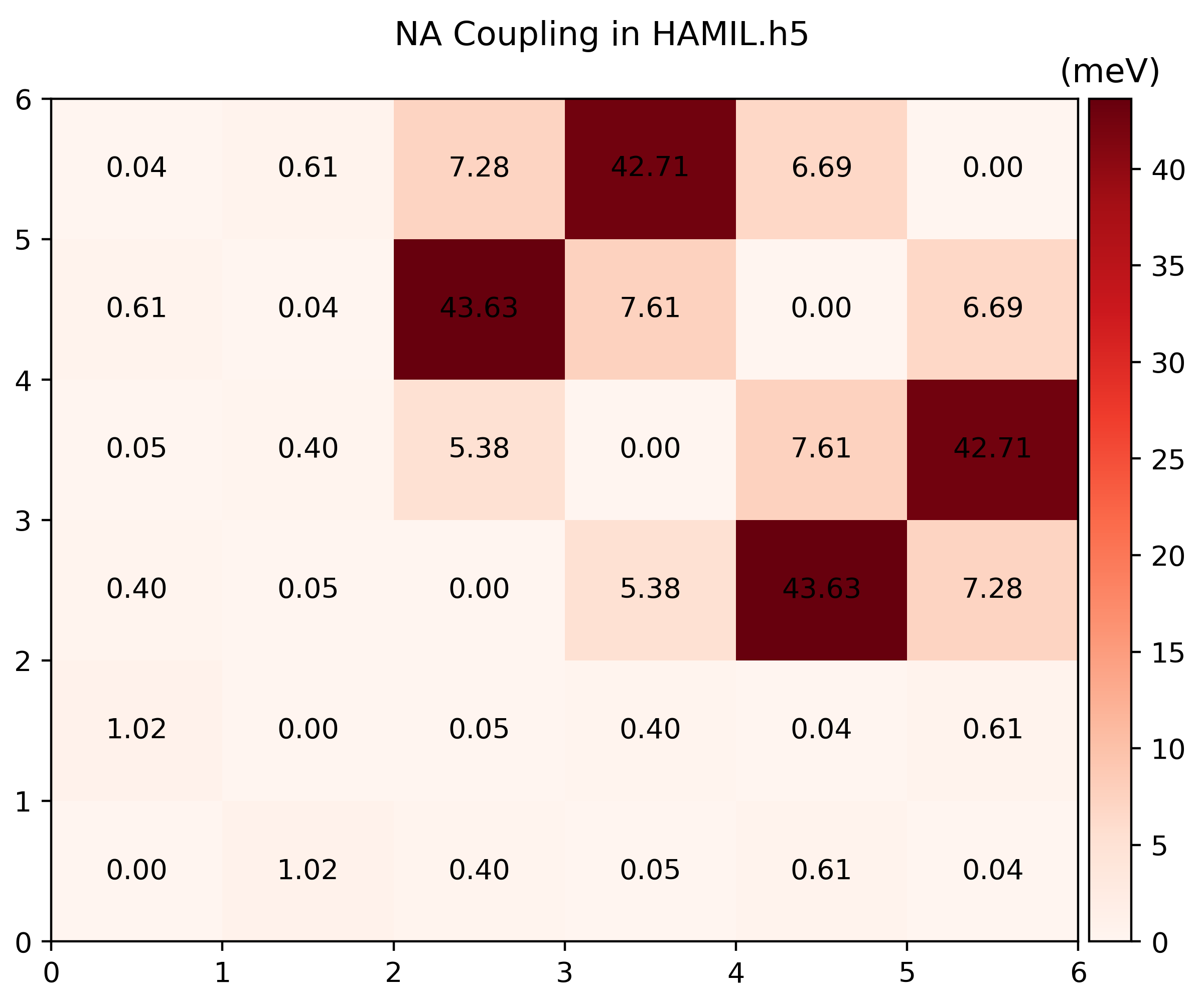
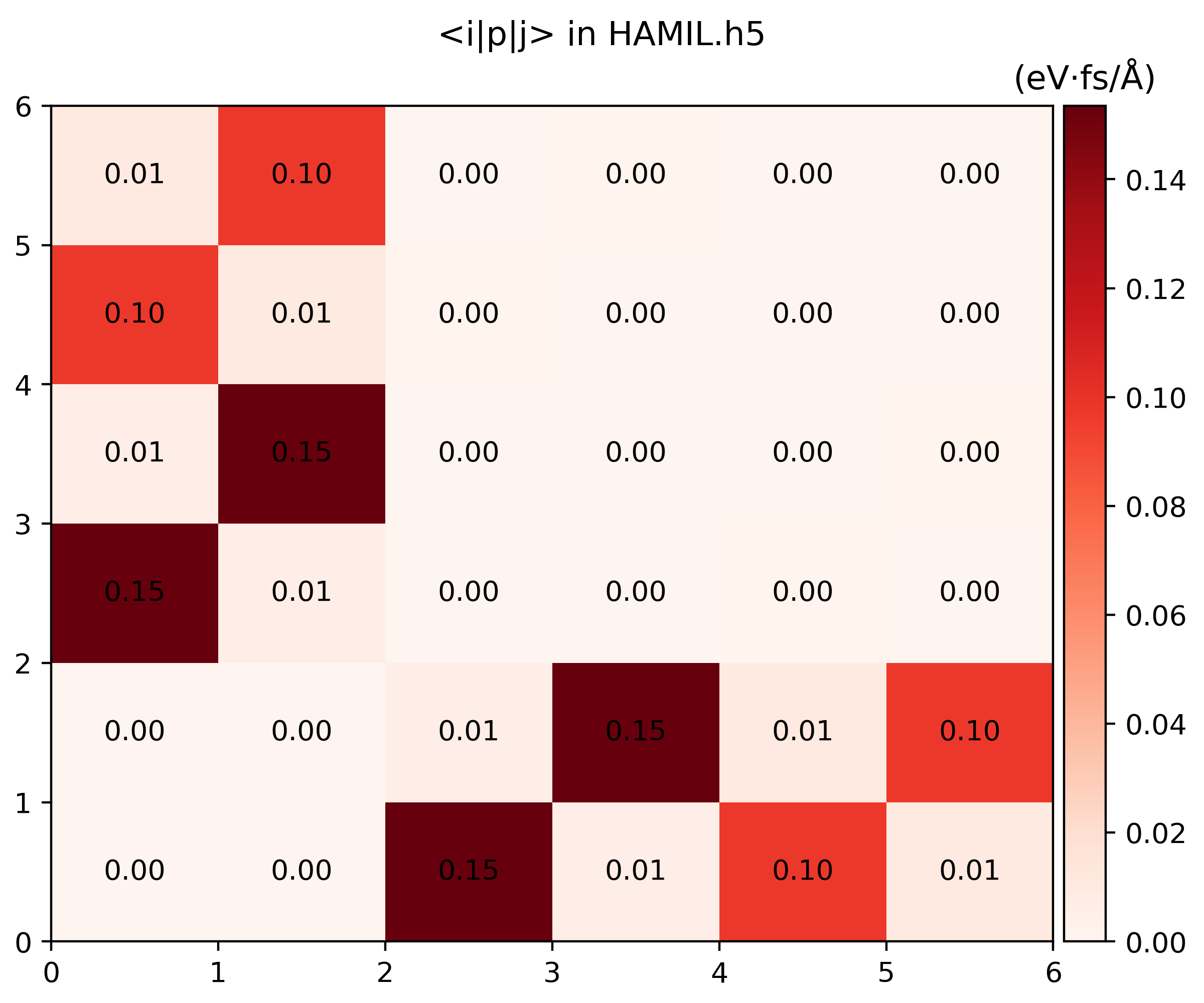
   Run namd_lmi hamil --generate pp to get hamil_plot.py, and then run it to get .pngs

   $ namd_lmi hamil --generate pp
   2024-11-20 16:07:04 [ INFO] Global logger initialized with targets being stderr and "./globalrun.log"
   2024-11-20 16:07:04 [ INFO] Writing `hamil_plot.py` ...
   2024-11-20 16:07:04 [ INFO] Time used: 1.868109ms
   
   $ python3 hamil_plot.py HAMIL.h5
   
   Writing hamil_nac.png
   Writing hamil_pij.png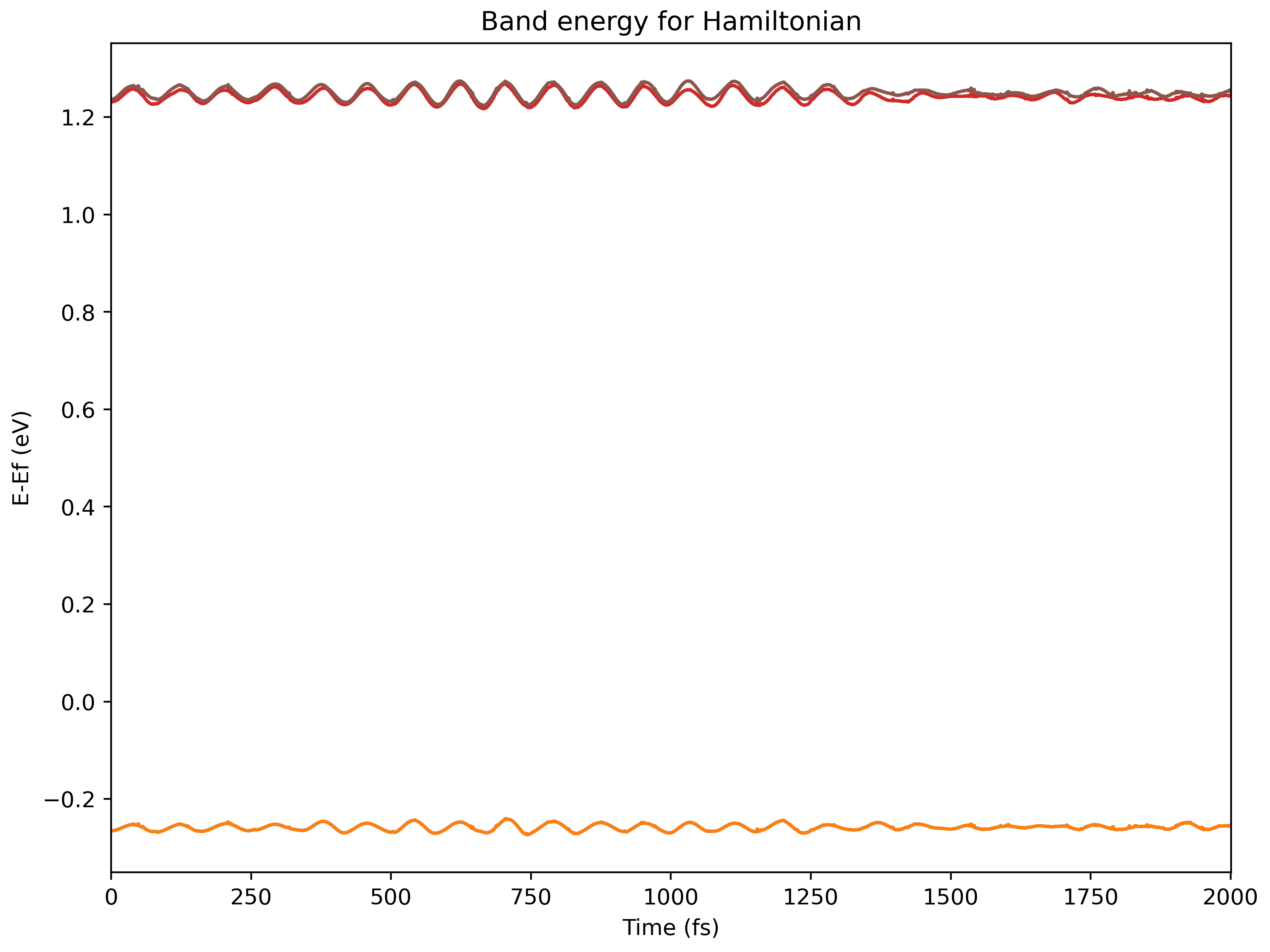
   

   

5. Data fields of HAMIL.h5

HDF5 "HAMIL.h5" {
GROUP "/" {
   DATASET "basis_labels" {
      DATATYPE  H5T_STD_U8LE
      DATASPACE  SIMPLE { ( 31 ) / ( 31 ) }
   }
   DATASET "basis_list" {
      DATATYPE  H5T_STD_I32LE
      DATASPACE  SIMPLE { ( 6 ) / ( 6 ) }
   }
   DATASET "efield" {
      DATATYPE  H5T_STD_U8LE
      DATASPACE  SIMPLE { ( 2263 ) / ( 2263 ) }
   }
   DATASET "eig_t" {
      DATATYPE  H5T_IEEE_F64LE
      DATASPACE  SIMPLE { ( 1999, 6 ) / ( 1999, 6 ) }
   }
   DATASET "ikpoint" {
      DATATYPE  H5T_STD_U64LE
      DATASPACE  SCALAR
   }
   DATASET "nac_t_i" {
      DATATYPE  H5T_IEEE_F64LE
      DATASPACE  SIMPLE { ( 1999, 6, 6 ) / ( 1999, 6, 6 ) }
   }
   DATASET "nac_t_r" {
      DATATYPE  H5T_IEEE_F64LE
      DATASPACE  SIMPLE { ( 1999, 6, 6 ) / ( 1999, 6, 6 ) }
   }
   DATASET "nbasis" {
      DATATYPE  H5T_STD_U64LE
      DATASPACE  SCALAR
   }
   DATASET "ndigit" {
      DATATYPE  H5T_STD_U64LE
      DATASPACE  SCALAR
   }
   DATASET "nsw" {
      DATATYPE  H5T_STD_U64LE
      DATASPACE  SCALAR
   }
   DATASET "pij_t_i" {
      DATATYPE  H5T_IEEE_F64LE
      DATASPACE  SIMPLE { ( 1999, 3, 6, 6 ) / ( 1999, 3, 6, 6 ) }
   }
   DATASET "pij_t_r" {
      DATATYPE  H5T_IEEE_F64LE
      DATASPACE  SIMPLE { ( 1999, 3, 6, 6 ) / ( 1999, 3, 6, 6 ) }
   }
   DATASET "potim" {
      DATATYPE  H5T_IEEE_F64LE
      DATASPACE  SCALAR
   }
   DATASET "proj_t" {
      DATATYPE  H5T_IEEE_F64LE
      DATASPACE  SIMPLE { ( 1999, 6, 36, 9 ) / ( 1999, 6, 36, 9 ) }
   }
   DATASET "propmethod" {
      DATATYPE  H5T_STD_U8LE
      DATASPACE  SIMPLE { ( 4 ) / ( 4 ) }
   }
   DATASET "scissor" {
      DATATYPE  H5T_IEEE_F64LE
      DATASPACE  SCALAR
   }
   DATASET "temperature" {
      DATATYPE  H5T_IEEE_F64LE
      DATASPACE  SCALAR
   }
}
}

Surface Hopping

This is the "literal" running process to simulate the dynamics of carriers. It ultilizes the Fewest switches surface hopping (FSSH) algorithm under the classical path approximation (CPA) to estimate the real-time population of each state. The hopping probability reads

\begin{equation} P_{j\to k}(t, t+\Delta t) = \max \qty{-2 \Delta t \qty( -\frac{\Re(\rho_{jk} D_{jk})}{\rho_{jj}} + \frac{ \Re(\rho_{jk} H_{jk}^{LMI} / i\hbar)}{\rho_{jj}} ), 0} \end{equation}

The formalism of FSSH is consistent with previous studies:

• J. Chem. Theory Comput. 2013, 9, 11, 4959–4972
• J. Chem. Theory Comput. 2014, 10, 2, 789–804
• WIREs Comput Mol Sci. 2019;9:e1411.

Help message

$ namd_lmi surfhop --help
Perform the surface-hopping process with given Hamiltonian file and config file

Usage: namd_lmi surfhop [OPTIONS]

Options:
  -n, --nthreads <NTHREADS>
          Number of threads for parallel calculation.

          If 0 is set, it will fall back to the number of logic CPU cores of you machine.

          [default: 0]

  -c, --config <CONFIG>
          Config file name.

          Aliases: "cfg", "conf".

      --generate <GENERATE>
          Generate auxiliary files for the calculation and analysis.

          The surface-hopping will not run if this flag is set.

          Alias: "gen".

          Possible values:
          - config-template:      Generate config template for Hamiltonian generation. Aliases: "config", "cfg" and "conf"
          - inistep.py:           Generate Python script to help append `inistep` field. Aliases: "inistep" and "ini"
          - postprocess-template: Generate post-process scripts for surface-hopping analysis. Aliases: "post-process", "postprocess", "pp"

      --collect-results <COLLECT_RESULTS>
          Collect results produced by the surface-hopping.

          The surface-hopping will not run if this flag is set.

          Aliases: "collect", "cr"

  -h, --help
          Print help (see a summary with '-h')

Procedures

1. Generate configuration file, and auxiliary Python script.

   $ namd_lmi surfhop --generate conf
   2024-11-20 20:59:21 [ INFO] Global logger initialized with targets being stderr and "./globalrun.log"
   2024-11-20 20:59:21 [ INFO] writing `03_surfhop_config_template.toml` ...
   2024-11-20 20:59:21 [ INFO] Writing `inisteps.py` ...
   2024-11-20 20:59:21 [ INFO] Time used: 13.977617ms
   
   $ namd_lmi surfhop --generate pp
   2024-11-20 20:59:30 [ INFO] Global logger initialized with targets being stderr and "./globalrun.log"
   2024-11-20 20:59:30 [ INFO] Writing `surfhop_plot.py` ...
   2024-11-20 20:59:30 [ INFO] Time used: 1.534094ms
   

2. Modify the Surface Hopping configuration file

   ####             NAMD-lmi config for surface-hopping calculation            ####
   #### YOUT NEED TO CHANGE THE PARAMETERS IN THE FOLLOWING TO FIT YOUR SYSTEM ####
   
             hamil_fname = "HAMIL.h5"
                namdtime = 1000
                    nelm = 10
                   ntraj = 10000
                shmethod = "FSSH"
   
                  outdir = "outdir"
        detailed_balance = "DependsOnEField"
         smearing_method = "LorentzianSmearing"
          smearing_sigma = 0.01
    smearing_npoints_per_eV = 500
   
                 iniband = "0"
                inisteps = [
            1 ,
            2 ,
            3 ,
   ]
   

   Explanation of each field:

   • hamil_fname string: Hamiltonian file name.

   • namdtime integer: Total NAMD simulate steps.

   • nelm integer: How many electronic steps within each ionic step.

     For propmethod = "FiniteDifference" in Hamiltonian, this field is required to be large, i.e. nelm = 1000. Otherwise, nelm = 10 is enough.

   • ntraj integer: How many times to hop for each MD trajectory.

   • shmethod string: Which surface hopping method to use. Only "FSSH" is available for now.

   • outdir string: Output directory where the results will be written in. This field cannot be current dir ".".

   • detailed_balance string: When the "detailed balance" factor \(B = e^{\Delta E / k_B T}\) applied on the upward hopping (hopping from lower energy to higher energy) probability.

     Available options:

     • "Always": Always apply factor \(B\).
     • "DependsOnEfield": Apply factor \(B\) only when external field is present, to allow upward hoppings.
     • "NacOnly": Apply factor \(B\) only for NAC driven upward hoppings, meaning that only phonon (plus SOC) induced upward hoppings are restricted.
     • "Never": Never apply this factor, no limitation on all upward hoppings.

   • smearing_method string: Smearing function for phonon spectra calculation.

     Available options:

     • "LorentzianSmearing"/"Lorentzian"/"lorentzian"
     • "GaussianSmearing"/"Gaussian"/"gaussian"

   • smearing_sigma float: Literal smearing width of smearing functions.

   • smearing_npoints_per_eV integer: Point density for spectra data.

   • iniband string: Bands where the electrons initially lie on. The indices is consistent with nac and hamil. Format is same as basis_list.

     For example, if basis_list = "215..220", and we want the electron on band 220 initially, this field should be iniband = "220"; if we want three electrons on band 215, 216 and 217 respectively, the this field should be iniband = "215..217".

   • inisteps list of integer: Initial step index for each NAMD sample trajectory.

     There are only 3 samples as shown in inisteps field, which is far from enough. Run python3 inisteps.py 03_surfhop_config_template.toml 1999 100 to generate 100 random initial configurations for the surface hopping method. Then delete the original inisteps and it finally reads

     ...
     ...
      smearing_npoints_per_eV = 500
     
                   iniband = 0
     ## Appended by inisteps.py @ 2024-11-20 22:42:28
                 inisteps = [
             13 ,
             64 ,
             78 ,
     ...
     ...
           1965 ,
           1982 ,
           1993
     ]
     

3. Run the surface hopping.

$ namd_lmi surfhop -c 03_surfhop_config_template.toml
2024-11-21 10:08:20 [ INFO] Global logger initialized with targets being stderr and "./globalrun.log"
2024-11-21 10:08:20 [ INFO]
+----------------------------------------------------------------------+
|                                                                      |
|    _   _            __  __  _____           _       __  __  _____    |
|   | \ | |    /\    |  \/  ||  __ \         | |     |  \/  ||_   _|   |
|   |  \| |   /  \   | \  / || |  | | ______ | |     | \  / |  | |     |
|   | . ` |  / /\ \  | |\/| || |  | ||______|| |     | |\/| |  | |     |
|   | |\  | / ____ \ | |  | || |__| |        | |____ | |  | | _| |_    |
|   |_| \_|/_/    \_\|_|  |_||_____/         |______||_|  |_||_____|   |
|                                                                      |
+----------------------------------------------------------------------+

Welcome to use namd!
    current version:    0.1.0
    git hash:           a51d001
    author(s):          Ionizing
    host:               x86_64-unknown-linux-gnu
    built time:         2024-11-20 16:02:14 +08:00

2024-11-21 10:08:20 [ INFO] Prepare to run surface-hopping in 0 threads ...
2024-11-21 10:08:20 [ INFO] Log and output files will be stored in "outdir" .
2024-11-21 10:08:20 [ INFO] Got Surface Hopping config:
####             NAMD-lmi config for surface-hopping calculation            ####
#### YOUT NEED TO CHANGE THE PARAMETERS IN THE FOLLOWING TO FIT YOUR SYSTEM ####

          hamil_fname = "HAMIL.h5"
             namdtime = 1000
                 nelm = 10
                ntraj = 10000
             shmethod = "FSSH"

               outdir = "outdir"
     detailed_balance = "DependsOnEField"
      smearing_method = "LorentzianSmearing"
       smearing_sigma = 0.01
 smearing_npoints_per_eV = 500

              iniband = 220
             inisteps = [
        13 ,
        64 ,
        78 ,
...
...
      1965 ,
      1982 ,
      1993 ,
]

2024-11-21 10:08:20 [ INFO] Linking Hamiltonian file "HAMIL.h5" to "outdir"
2024-11-21 10:08:20 [ INFO] Writing electric field source file to efield.rhai ...
2024-11-21 10:08:20 [ INFO] Writing electric field to "outdir/EAFIELD.txt" ...
2024-11-21 10:08:20 [ INFO] Running surface hopping with namdinit = 81 ...
2024-11-21 10:08:20 [ INFO] Running surface hopping with namdinit = 625 ...
2024-11-21 10:08:20 [ INFO] Running surface hopping with namdinit = 896 ...
...
...
2024-11-21 10:08:22 [ INFO] Running surface hopping with namdinit = 457 ...
2024-11-21 10:08:22 [ INFO] Running surface hopping with namdinit = 478 ...
2024-11-21 10:08:22 [ INFO] Running surface hopping with namdinit = 430 ...
2024-11-21 10:08:22 [ INFO] Collecting results ...
2024-11-21 10:08:22 [ INFO] Processing "outdir/result_0013.h5" ...
2024-11-21 10:08:22 [ INFO] Processing "outdir/result_0081.h5" ...
2024-11-21 10:08:22 [ INFO] Processing "outdir/result_0925.h5" ...
...
...
2024-11-21 10:08:23 [ INFO] Processing "outdir/result_1872.h5" ...
2024-11-21 10:08:23 [ INFO] Processing "outdir/result_0689.h5" ...
2024-11-21 10:08:23 [ INFO] Processing "outdir/result_1529.h5" ...
2024-11-21 10:08:23 [ INFO] Collecting done. Writing to "outdir/averaged_results.h5" ...
2024-11-21 10:08:23 [ INFO] Time used: 3.848758855s

4. Visualize results

Generate the visualization script and then run it.

$ namd_lmi surfhop --generate pp
2024-11-21 10:12:03 [ INFO] Global logger initialized with targets being stderr and "./globalrun.log"
2024-11-21 10:12:03 [ INFO] Writing `surfhop_plot.py` ...
2024-11-21 10:12:03 [ INFO] Time used: 1.444398ms

$ cd outdir && python3 ../surfhop_plot.py
03_surfhop_config_template.toml  result_0282.h5  result_0625.h5  result_0859.h5  result_1240.h5  result_1656.h5
averaged_results.h5              result_0291.h5  result_0669.h5  result_0896.h5  result_1263.h5  result_1658.h5
EAFIELD.txt                      result_0293.h5  result_0680.h5  result_0925.h5  result_1297.h5  result_1715.h5
efield.rhai                      result_0301.h5  result_0685.h5  result_0947.h5  result_1309.h5  result_1733.h5
HAMIL.h5                         result_0302.h5  result_0686.h5  result_0949.h5  result_1310.h5  result_1745.h5
result_0013.h5                   result_0311.h5  result_0689.h5  result_0979.h5  result_1326.h5  result_1764.h5
result_0064.h5                   result_0336.h5  result_0725.h5  result_1014.h5  result_1336.h5  result_1834.h5
result_0078.h5                   result_0365.h5  result_0726.h5  result_1019.h5  result_1376.h5  result_1872.h5
result_0081.h5                   result_0429.h5  result_0749.h5  result_1020.h5  result_1382.h5  result_1886.h5
result_0087.h5                   result_0430.h5  result_0758.h5  result_1023.h5  result_1416.h5  result_1923.h5
result_0099.h5                   result_0457.h5  result_0759.h5  result_1049.h5  result_1432.h5  result_1950.h5
result_0153.h5                   result_0478.h5  result_0760.h5  result_1064.h5  result_1435.h5  result_1957.h5
result_0154.h5                   result_0508.h5  result_0789.h5  result_1072.h5  result_1522.h5  result_1965.h5
result_0183.h5                   result_0524.h5  result_0790.h5  result_1078.h5  result_1529.h5  result_1982.h5
result_0207.h5                   result_0541.h5  result_0792.h5  result_1091.h5  result_1532.h5  result_1993.h5
result_0214.h5                   result_0546.h5  result_0817.h5  result_1119.h5  result_1572.h5  run.log
result_0238.h5                   result_0549.h5  result_0818.h5  result_1133.h5  result_1587.h5  surfhop.png
result_0244.h5                   result_0618.h5  result_0837.h5  result_1159.h5  result_1616.h5  wfn_propagation.png

The coefficient propagation should looks like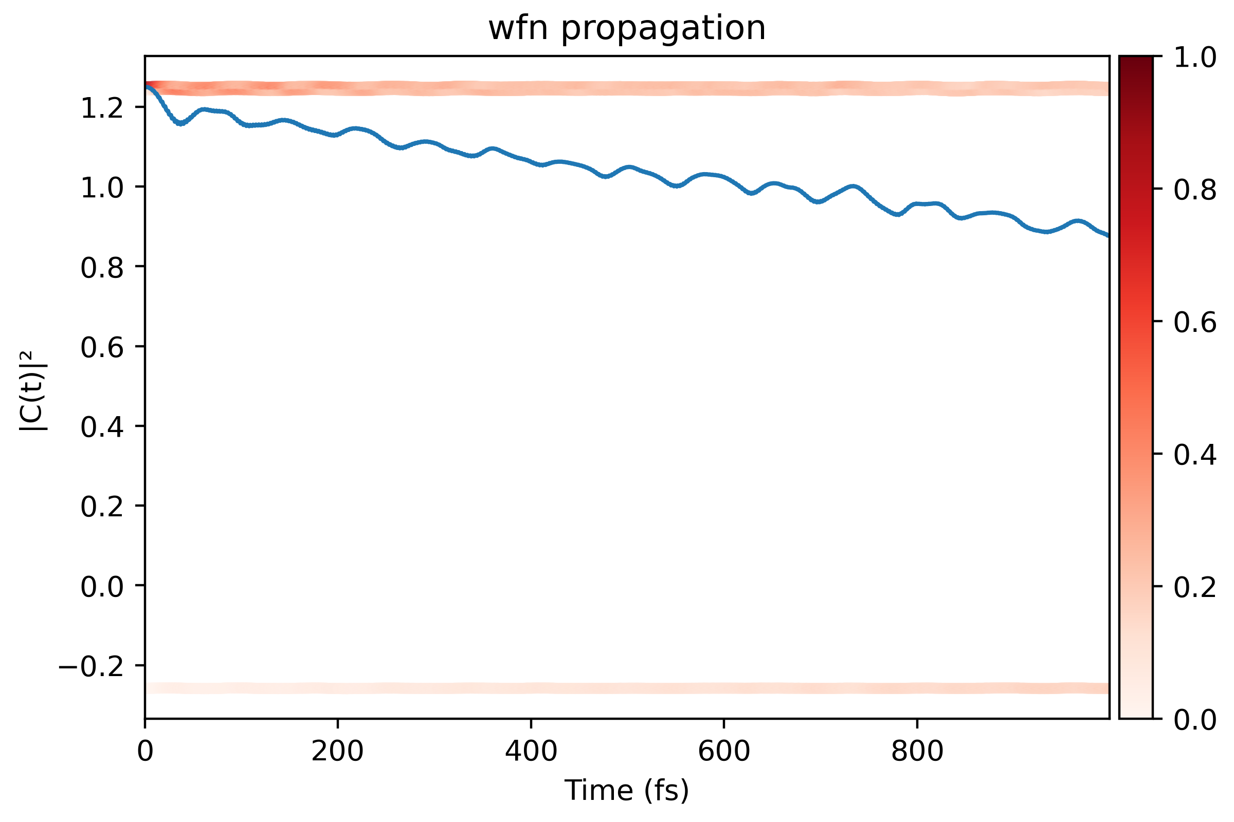

And the surface hopping result looks like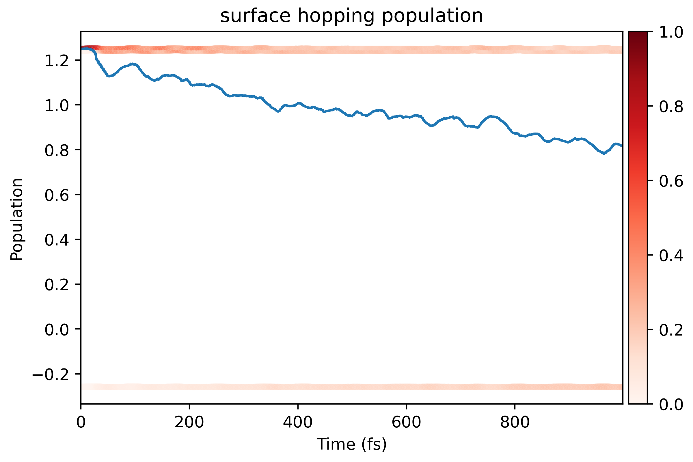

Data fields of result_xxxx.h5 and averaged_results.h5

$ h5dump -H result_0013.h5
HDF5 "result_0013.h5" {
GROUP "/" {
   DATASET "basis_labels" {
      DATATYPE  H5T_STD_U8LE
      DATASPACE  SIMPLE { ( 31 ) / ( 31 ) }
   }
   DATASET "basis_list" {
      DATATYPE  H5T_STD_I32LE
      DATASPACE  SIMPLE { ( 6 ) / ( 6 ) }
   }
   DATASET "detailed_balance" {
      DATATYPE  H5T_STD_U8LE
      DATASPACE  SIMPLE { ( 15 ) / ( 15 ) }
   }
   DATASET "namdinit" {
      DATATYPE  H5T_STD_U64LE
      DATASPACE  SCALAR
   }
   DATASET "namdtime" {
      DATATYPE  H5T_STD_U64LE
      DATASPACE  SCALAR
   }
   DATASET "ntraj" {
      DATATYPE  H5T_STD_U64LE
      DATASPACE  SCALAR
   }
   DATASET "prop_energy" {
      DATATYPE  H5T_IEEE_F64LE
      DATASPACE  SIMPLE { ( 1000 ) / ( 1000 ) }
   }
   DATASET "psi_t_i" {
      DATATYPE  H5T_IEEE_F64LE
      DATASPACE  SIMPLE { ( 1000, 6 ) / ( 1000, 6 ) }
   }
   DATASET "psi_t_r" {
      DATATYPE  H5T_IEEE_F64LE
      DATASPACE  SIMPLE { ( 1000, 6 ) / ( 1000, 6 ) }
   }
   DATASET "sh_energy" {
      DATATYPE  H5T_IEEE_F64LE
      DATASPACE  SIMPLE { ( 1000 ) / ( 1000 ) }
   }
   DATASET "sh_phonons_t" {
      DATATYPE  H5T_IEEE_F64LE
      DATASPACE  SIMPLE { ( 1000, 6, 6 ) / ( 1000, 6, 6 ) }
   }
   DATASET "sh_photons_t" {
      DATATYPE  H5T_IEEE_F64LE
      DATASPACE  SIMPLE { ( 1000, 6, 6 ) / ( 1000, 6, 6 ) }
   }
   DATASET "sh_pops" {
      DATATYPE  H5T_IEEE_F64LE
      DATASPACE  SIMPLE { ( 1000, 6 ) / ( 1000, 6 ) }
   }
   DATASET "shmethod" {
      DATATYPE  H5T_STD_U8LE
      DATASPACE  SIMPLE { ( 5 ) / ( 5 ) }
   }
   DATASET "time" {
      DATATYPE  H5T_IEEE_F64LE
      DATASPACE  SIMPLE { ( 1000 ) / ( 1000 ) }
   }
}
}

$ h5dump -H averaged_results.h5
HDF5 "averaged_results.h5" {
GROUP "/" {
   DATASET "basis_labels" {
      DATATYPE  H5T_STD_U8LE
      DATASPACE  SIMPLE { ( 31 ) / ( 31 ) }
   }
   DATASET "basis_list" {
      DATATYPE  H5T_STD_I32LE
      DATASPACE  SIMPLE { ( 6 ) / ( 6 ) }
   }
   DATASET "delta_et" {
      DATATYPE  H5T_IEEE_F64LE
      DATASPACE  SIMPLE { ( 21, 1999 ) / ( 21, 1999 ) }
   }
   DATASET "eigs_t" {
      DATATYPE  H5T_IEEE_F64LE
      DATASPACE  SIMPLE { ( 1000, 6 ) / ( 1000, 6 ) }
   }
   DATASET "ndigit" {
      DATATYPE  H5T_STD_U64LE
      DATASPACE  SCALAR
   }
   DATASET "phonon_spectra_frequencies" {
      DATATYPE  H5T_IEEE_F64LE
      DATASPACE  SIMPLE { ( 1000 ) / ( 1000 ) }
   }
   DATASET "phonons_absp_t" {
      DATATYPE  H5T_IEEE_F64LE
      DATASPACE  SIMPLE { ( 1000, 1000 ) / ( 1000, 1000 ) }
   }
   DATASET "phonons_emit_t" {
      DATATYPE  H5T_IEEE_F64LE
      DATASPACE  SIMPLE { ( 1000, 1000 ) / ( 1000, 1000 ) }
   }
   DATASET "phonons_spectra" {
      DATATYPE  H5T_IEEE_F64LE
      DATASPACE  SIMPLE { ( 21, 1000 ) / ( 21, 1000 ) }
   }
   DATASET "photon_spectra_xvals" {
      DATATYPE  H5T_IEEE_F64LE
      DATASPACE  SIMPLE { ( 1400 ) / ( 1400 ) }
   }
   DATASET "photons_absp_t" {
      DATATYPE  H5T_IEEE_F64LE
      DATASPACE  SIMPLE { ( 1000, 1400 ) / ( 1000, 1400 ) }
   }
   DATASET "photons_emit_t" {
      DATATYPE  H5T_IEEE_F64LE
      DATASPACE  SIMPLE { ( 1000, 1400 ) / ( 1000, 1400 ) }
   }
   DATASET "potim" {
      DATATYPE  H5T_IEEE_F64LE
      DATASPACE  SCALAR
   }
   DATASET "proj_t" {
      DATATYPE  H5T_IEEE_F64LE
      DATASPACE  SIMPLE { ( 1000, 6, 36, 9 ) / ( 1000, 6, 36, 9 ) }
   }
   DATASET "prop_energy" {
      DATATYPE  H5T_IEEE_F64LE
      DATASPACE  SIMPLE { ( 1000 ) / ( 1000 ) }
   }
   DATASET "psi_t" {
      DATATYPE  H5T_IEEE_F64LE
      DATASPACE  SIMPLE { ( 1000, 6 ) / ( 1000, 6 ) }
   }
   DATASET "sh_energy" {
      DATATYPE  H5T_IEEE_F64LE
      DATASPACE  SIMPLE { ( 1000 ) / ( 1000 ) }
   }
   DATASET "sh_phonons_t" {
      DATATYPE  H5T_IEEE_F64LE
      DATASPACE  SIMPLE { ( 1000, 6, 6 ) / ( 1000, 6, 6 ) }
   }
   DATASET "sh_photons_t" {
      DATATYPE  H5T_IEEE_F64LE
      DATASPACE  SIMPLE { ( 1000, 6, 6 ) / ( 1000, 6, 6 ) }
   }
   DATASET "sh_pops" {
      DATATYPE  H5T_IEEE_F64LE
      DATASPACE  SIMPLE { ( 1000, 6 ) / ( 1000, 6 ) }
   }
   DATASET "time" {
      DATATYPE  H5T_IEEE_F64LE
      DATASPACE  SIMPLE { ( 1000 ) / ( 1000 ) }
   }
}
}

Feedback

We are happy that you reach here. As an open-source project, NAMD-LMI welcomes feedback.

• If you want to add features to NAMD-LMI, just open an issue at GitHub Issues. We also created a feature-requests list, you can follow it at this page.

• If namd_lmi complains something or produces wrong result, just open an issue at GitHub Issues. We are grateful if you can provide the input files in order that we can reproduce the issue conveniently, thus solve the issue as soon as possible.

• If you are interested in NAMD-LMI and want to contribute to the source code, just fork NAMD-LMI and create pull requests at Pull Requests. We are super grateful if you can contribute to NAMD-LMI.

Acknowledgements

• Prof. Jin Zhao
• Prof. Qijing Zheng
• Hefei-NAMD
• Dr. Zhi Li
• CN Rust User Group